![]()
in which gravitational waves carry to Earth
encoded symphonies of black holes colliding,
and physicists devise instruments
to monitor the waves
and decipher their symphonies
Symphonies
I n the core of a far-off galaxy, a billion light-years from Earth and a billion years ago, there accumulated a dense agglomerate of gas and hundreds of millions of stars. The agglomerate gradually shrank, as one star after another was flung out and the remaining 100 million stars sank closer to the center. After 100 million years, the agglomerate had shrunk to several light-years in size, and small stars began, occasionally, to collide and coalesce, forming larger stars. The larger stars consumed their fuel and then imploded to form black holes, and pairs of holes, flying close to each other, occasionally were captured into orbit around each other.
Figure 10.1 shows an embedding diagram for one such black-hole binary. Each hole creates a deep pit (strong spacetime curvature) in the embedded surface, and as the holes encircle each other, the orbiting pits produce ripples of curvature that propagate outward with the speed of light. The ripples form a spiral in the fabric of spacetime around the binary, much like the spiraling pattern of water from a rapidly rotating lawn sprinkler. Just as each drop of water from the sprinkler flies nearly radially outward, so each bit of curvature flies nearly radially outward; and just as the outward flying drops together form a spiraling stream of water, so all the bits of curvature together form spiraling ridges and valleys in the fabric of spacetime.
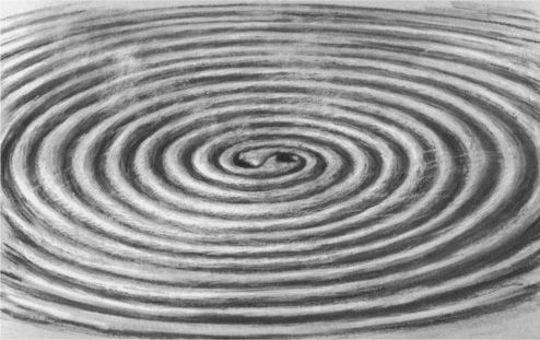
10.1 An embedding diagram depicting the curvature of space in the orbital “plane” of a binary system made of two black holes. At the center are two pits that represent the strong spacetime curvature around the two holes. These pits are the same as encountered in previous black-hole embedding diagrams, for example, Figure 7.6. As the holes orbit each other, they create outward propagating ripples of curvature called gravitational waves. [Courtesy LIGO Project, California Institute of Technology.]
Since spacetime curvature is the same thing as gravity, these ripples of curvature are actually waves of gravity, or gravitational waves. Einstein’s general theory of relativity predicts, unequivocally, that such gravitational waves must be produced whenever two black holes orbit each other—and also whenever two stars orbit each other.
As they depart for outer space, the gravitational waves push back on the holes in much the same way as a bullet kicks back on the gun that fires it. The waves’ push drives the holes closer together and up to higher speeds; that is, it makes them slowly spiral inward toward each other. The inspiral gradually releases gravitational energy, with half of the released energy going into the waves and the other half into increasing the holes’ orbital speeds.
The holes’ inspiral is slow at first, but the closer the holes draw to each other, the faster they move, the more strongly they radiate their ripples of curvature, and the more rapidly they lose energy and spiral inward (Figures 10.2a,b). Ultimately, when each hole is moving at nearly the speed of light, their horizons touch and merge. Where once there were two holes, now there is one—a rapidly spinning, dumbbell-shaped hole (Figure 10.2c). As the horizon spins, its dumbbell shape radiates ripples of curvature, and those ripples push back on the hole, gradually reducing its dumbbell protrusions until they are gone (Figure 10.2d). The spinning hole’s horizon is left perfectly smooth and circular in equatorial cross section, with precisely the shape described by Kerr’s solution to the Einstein field equation (Chapter 7 ).
By examining the final, smooth black hole, one cannot in any way discover its past history. One cannot discern whether it was created by the coalescence of two smaller holes, or by the direct implosion of a star made of matter, or by the direct implosion of a star made of antimatter. The black hole has no “hair” from which to decipher its history (Chapter 7 ).
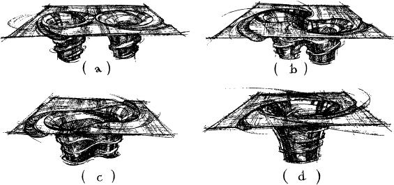
10.2 Embedding diagrams depicting the curvature of space around a binary system made of two black holes. The diagrams have been embellished by the artist to give a sense of motion. Each successive diagram is at a later moment of time, when the two holes have spiraled closer together. In diagrams (a) and (b), the holes’ horizons are the circles at the bottoms of the pits. The horizons merge just before diagram (c), to form a single, dumbbell-shaped horizon. The rotating dumbbell emits gravitational waves, which carry away its deformation, leaving behind a smooth, spinning, Kerr black hole in diagram (d). [Courtesy LIGO Project, California Institute of Technology.]
However, the history is not entirely lost. A record has been kept: It has been encoded in the ripples of spacetime curvature that the coalescing holes emitted. Those curvature ripples are much like the sound waves from a symphony. Just as the symphony is encoded in the sound waves’ modulations (larger amplitude here, smaller there; higher frequency wiggles here, lower there), so the coalescence history is encoded in modulations of the curvature ripples. And just as the sound waves carry their encoded symphony from the orchestra that produces it to the audience, so the curvature ripples carry their encoded history from the coalescing holes to the distant Universe.
The curvature ripples travel outward in the fabric of spacetime, through the agglomerate of stars and gas where the two holes were born. The agglomerate absorbs none of the ripples and distorts them not at all; the ripples’ encoded history remains perfectly unchanged. On outward the ripples propagate, through the agglomerate’s parent galaxy and into intergalactic space, through the cluster of galaxies in which the parent galaxy resides, then onward through one cluster of galaxies after another and into our own cluster, into our own Milky Way galaxy, and into our solar system, through the Earth, and on out toward other, distant galaxies.
If we humans are clever enough, we should be able to monitor the ripples of spacetime curvature as they pass. Our computers can translate them from ripples of curvature to ripples of sound, and we then will hear the holes’ symphony: a symphony that gradually rises in pitch and intensity as the holes spiral together, then gyrates in a wild way as they coalesce into one, deformed hole, then slowly fades with steady pitch as the hole’s protrusions gradually shrink and disappear.
If we can decipher it, the ripples’ symphony will contain a wealth of information:
1. The symphony will contain a signature that says, “I come from a pair of black holes that are spiraling together and coalescing.” This will be the kind of absolutely unequivocal black-hole signature that astronomers thus far have searched for in vain using light and X-rays ( Chapter 8 ) and radio waves ( Chapter 9 ). Because the light, X-rays, and radio waves are produced far outside a hole’s horizon, and because they are emitted by a type of material (hot, high-speed electrons) that is completely different from that of which the hole is made (pure spacetime curvature), and because they can be strongly distorted by propagating through intervening matter, they can bring us but little information about the hole, and no definitive signature. The ripples of curvature (gravitational waves), by contrast, are produced very near the coalescing holes’ horizons, they are made of the same material (a warpage of the fabric of spacetime) as the holes, they are not distorted at all by propagating through intervening matter—and, as a consequence, they can bring us detailed information about the holes and an unequivocal black-hole signature.
2. The ripples’ symphony can tell us just how heavy each of the holes was, how fast they were spinning, the shape of their orbit (circular? elongated?), where the holes are on our sky, and how far they are from Earth.
3. The symphony will contain a partial map of the inspiraling holes’ spacetime curvature. For the first time we will be able to test definitively general relativity’s black-hole predictions: Does the symphony’s map agree with Kerr’s solution of the Einstein field equation ( Chapter 7 )? Does the map show space swirling near the spinning hole, as Kerr’s solution demands? Does the amount of swirl agree with Kerr’s solution? Does the way the swirl changes as one approaches the horizon agree with Kerr’s solution?
4. The symphony will describe the merging of the two holes’ horizons and the wild vibrations of the newly merged holes—merging and vibrations of which, today, we have only the vaguest understanding. We understand them only vaguely because they are governed by a feature of Einstein’s general relativity laws that we comprehend only poorly: the laws’ nonlinearity (Box 10.1). By “nonlinearity” is meant the propensity of strong curvature itself to produce more curvature, which in turn produces still more curvature—much like the growth of an avalanche, where a trickle of sliding snow pulls new snow into the flow, which in turn grabs more snow until an entire mountainside of snow is in motion. We understand this nonlinearity in a quiescent black hole; there it is responsible for holding the hole together; it is the hole’s “glue.” But we do not understand what the nonlinearity does, how it behaves, what its effects are, when the strong curvature is violently dynamical. The merger and vibration of two holes is a promising “laboratory” in which to seek such understanding. The understanding can come through hand-in-hand cooperation between experimental physicists who monitor the symphonic ripples from coalescing holes in the distant Universe and theoretical physicists who simulate the coalescence on supercomputers.
Box 10.1
Nonlinearity and Its Consequences
A quantity is called linear if its total size is the sum of its parts; otherwise it is nonlinear.
My family income is linear: It is the sum of my wife’s salary and my own. The amount of money I have in my retirement fund is nonlinear: It is not the sum of all the contributions I have invested in the past; rather, it is far greater than that sum, because each contribution started earning interest when it was invested, and each bit of interest in turn earned interest of its own.
The volume of water flowing in a sewer pipe is linear: It is the sum of the contributions from all the homes that feed into the pipe. The volume of snow flowing in an avalanche is nonlinear: A tiny trickle of snow can trigger a whole mountainside of snow to start sliding.
Linear phenomena are simple, easy to analyze, easy to predict. Nonlinear phenomena are complex and hard to predict. Linear phenomena exhibit only a few types of behaviors; they are easy to categorize. Nonlinear phenomena exhibit great richness—a richness that scientists and engineers have only appreciated in recent years, as they have begun to confront a type of nonlinear behavior called chaos. (For a beautiful introduction to the concept of chaos see Gleick, 1987.)
When spacetime curvature is weak (as in the solar system), it is very nearly linear; for example, the tides on the Earth’s oceans are the sum of the tides produced by the Moon’s spacetime curvature (tidal gravity) and the tides produced by the Sun. By contrast, when spacetime curvature is strong (as in the big bang and near a black hole), Einstein’s general relativistic laws of gravity predict that the curvature should be extremely nonlinear—among the most nonlinear phenomena in the Universe. However, as yet we possess almost no experimental or observational data to show us the effects of gravitational nonlinearity, and we are so inept at solving Einstein’s equation that our solutions have taught us about the nonlinearity only in simple situations—for example, around a quiescent, spinning black hole.
A quiescent black hole owes its existence to gravitational nonlinearity; without the gravitational nonlinearity, the hole could not hold itself together, just as without gaseous nonlinearities, the great red spot on the planet Jupiter could not hold itself together. When the imploding star that creates a black hole disappears through the hole’s horizon, the star loses its ability to influence the hole in any way; most important, the star’s gravity can no longer hold the hole together. The hole then continues to exist solely because of gravitational nonlinearity: The hole’s spacetime curvature continuously regenerates itself nonlinearly, without the aid of the star; and the self-generated curvature acts as a nonlinear “glue” to bind itself together.
The quiescent black hole whets our appetites to learn more. What other phenomena can gravitational nonlinearity produce? Some answers may come from monitoring and decoding the ripples of spacetime curvature produced by coalescing black holes. We there might see chaotic, bizarre behaviors that we never anticipated.
T o achieve this understanding will require monitoring the holes’ symphonic ripples of curvature. How can they be monitored? The key is the physical nature of the curvature: Spacetime curvature is the same thing as tidal gravity. The spacetime curvature produced by the Moon raises tides in the Earth’s oceans (Figure 10.3a), and the ripples of spacetime curvature in a gravitational wave should similarly raise ocean tides (Figure 10.3b).
General relativity insists, however, that the ocean tides raised by the Moon and those raised by a gravitational wave differ in three major ways. The first difference is propagation. The gravitational wave’s tidal forces (curvature ripples) are analogous to light waves or radio waves: They travel from their source to the Earth at the speed of light, oscillating as they travel. The Moon’s tidal forces, by contrast, are like the electric field of a charged body. Just as the electric field is attached firmly to the charged body and the body carries it around, always sticking out of itself like quills out of a hedgehog, so also the tidal forces are attached firmly to the Moon, and the Moon carries them around, sticking out of itself in a never-changing way, ready always to grab hold of and squeeze and stretch anything that comes into the Moon’s vicinity. The Moon’s tidal forces squeeze and stretch the Earth’s oceans in a way that seems to change every few hours only because the Earth rotates through them. If the Earth did not rotate, the squeeze and stretch would be constant, unchanging.
The second difference is the direction of the tides (Figures 10.3a,b): The Moon produces tidal forces in all spatial directions. It stretches the oceans in the longitudinal direction (toward and away from the Moon), and it squeezes the oceans in transverse directions (perpendicular to the Moon’s direction). By contrast, a gravitational wave produces no tidal forces at all in the longitudinal direction (along the direction of the wave’s propagation). However, in the transverse plane, the wave stretches the oceans in one direction (the up–down direction in Figure 10.3b) and squeezes along the other direction (the front–back direction in Figure 10.3b). This stretch and squeeze is oscillatory. As a crest of the wave passes, the stretch is up-down, the squeeze is front–back; as a trough of the wave passes, there is a reversal to up–down squeeze and front–back stretch; as the next crest arrives, there is a reversal again to up–down stretch and front–back squeeze.
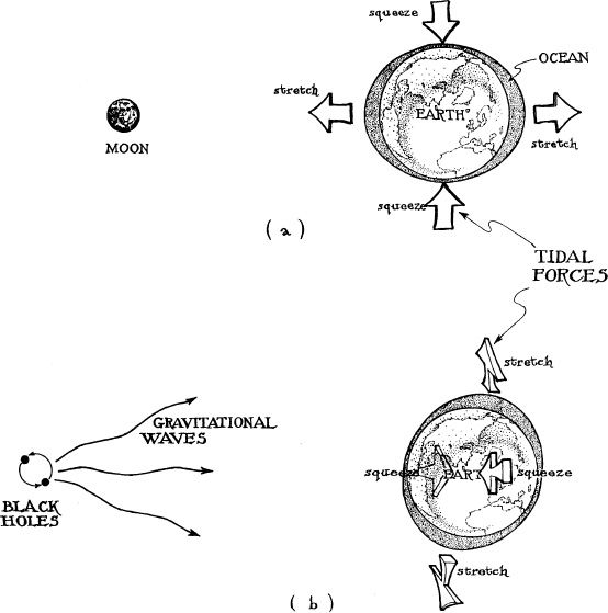
10.3 The tidal forces produced by the Moon and by a gravitational wave. (a) The Moon’s tidal forces stretch and squeeze the Earth’s oceans; the stretch is longitudinal, the squeeze is transverse. (b) A gravitational wave’s tidal forces stretch and squeeze the Earth’s oceans; the forces are entirely transverse, with a stretch along one transverse direction and a squeeze along the other.
The third difference between the Moon’s tides and those of a gravitational wave is their size. The Moon produces tides roughly 1 meter in size, so the difference between high tide and low tide is about 2 meters. By contrast, the gravitational waves from coalescing black holes should produce tides in the Earth’s oceans no larger than about 10 −14 meter, which is 10 −21 of the size of the Earth (and 1/10,000 the size of a single atom, and just 10 times larger than an atom’s nucleus). Since tidal forces are proportional to the size of the object on which they act (Chapter 2 ), the waves will tidally distort any object by about 10 −21 of its size. In this sense, 10 −21 is the strength of the waves when they arrive at Earth.
Why are the waves so weak? Because the coalescing holes are so far away. The strength of a gravitational wave, like the strength of a light wave, dies out inversely with the distance traveled. When the waves are still close to the holes, their strength is roughly 1; that is, they squeeze and stretch an object by about as much as the object’s size; humans would be killed by so strong a stretch and squeeze. However, when the waves have reached Earth, their strength is reduced to roughly (1/30 of the holes’ circumference) / (the distance the waves have traveled).
1
For holes that weigh about 10 times as much as the Sun and are a billion light-years away, this wave strength is (![]() ) × (180 kilometers for the horizon circumference)/(a billion lightyears for the distance to Earth)
) × (180 kilometers for the horizon circumference)/(a billion lightyears for the distance to Earth) ![]() 10
−21
. Therefore, the waves distort the Earth’s oceans by 10
−21
× (10
7
meters for the Earth’s size) = 10
−14
meter, or 10 times the diameter of an atomic nucleus.
10
−21
. Therefore, the waves distort the Earth’s oceans by 10
−21
× (10
7
meters for the Earth’s size) = 10
−14
meter, or 10 times the diameter of an atomic nucleus.
It is utterly hopeless to think of measuring such a tiny tide on the Earth’s turbulent ocean. Not quite so hopeless, however, are the prospects for measuring the gravitational wave’s tidal forces on a carefully designed laboratory instrument—a gravitational -wave detector.
Bars
J oseph Weber was the first person with sufficient insight to realize that it is not utterly hopeless to try to detect gravitational waves. A graduate of the D.S. Naval Academy in 1940 with a bachelor’s degree in engineering, Weber served in World War II on the aircraft carrier Lexington, until it was sunk in the Battle of the Coral Sea, and then became commanding officer of Submarine Chaser No. 690; and he led Brigadier General Theodore Roosevelt, Jr., and 1900 Rangers onto the beach in the 1943 invasion of Italy. After the war he became head of the electronic countermeasures section of the Bureau of Ships for the D.S. Navy. His reputation for mastery of radio and radar technology was so great that in 1948 he was offered and accepted the position of full professor of electrical engineering at the University of Maryland—full professor at age twenty-nine, and with no more college education than a bachelor’s degree.
While teaching electrical engineering at Maryland, Weber prepared for a career change: He worked toward, and completed, a Ph.D. in physics at Catholic University, in part under the same person as had been John Wheeler’s Ph.D. adviser, Karl Herzfeld. From Herzfeld, Weber learned enough about the physics of atoms, molecules, and radiation to invent, in 1951, one version of the mechanism by which lasers work, but he did not have the resources to demonstrate his concept experimentally. While Weber was publishing his concept, two other research groups, one at Columbia University led by Charles Townes and the other in Moscow led by Nikolai Gennadievich Basov and Aleksandr Michailovich Prokharov, independently invented alternative versions of the mechanism, and then went on to construct working lasers. 2 Though Weber’s paper had been the first publication on the mechanism, he received hardly any credit; the Nobel Prize and patents went to the Columbia and Moscow scientists. Disappointed, but maintaining close friendships with Townes and Basov, Weber sought a new research direction.
As part of his search, Weber spent a year in John Wheeler’s group, became an expert on general relativity, and with Wheeler did theoretical research on general relativity’s predictions of the properties of gravitational waves. By 1957, he had found his new direction. He would embark on the world’s first effort to build apparatus for detecting and monitoring gravitational waves.
Through late 1957, all of 1958, and early 1959, Weber struggled to invent every scheme he could for detecting gravitational waves. This was a pen, paper, and brainpower exercise, not experimental. He filled four 300-page notebooks with ideas, possible detector designs, and calculations of the expected performance of each design. One idea after another he cast aside as not promising. One design after another failed to give high sensitivity. But a few held promise; and of them, Weber ultimately chose a cylindrical aluminum bar about 2 meters long, a half meter in diameter, and a ton in weight, oriented broadside to the incoming waves (Figure 10.4 below).
As the waves’ tidal force oscillates, it should first compress, then stretch, then compress such a bar’s ends. The bar has a natural mode of vibration which can respond resonantly to this oscillating tidal force, a mode in which its ends vibrate in and out relative to its center. That natural mode, like the ringing of a bell or tuning fork or wine glass, has a well-defined frequency. Just as a bell or tuning fork or wine glass can be made to ring sympathetically by sound waves that match its natural frequency, so the bar can be made to vibrate sympathetically by oscillating tidal forces that match its natural frequency. To use such a bar as a gravitational-wave detector, then, one should adjust its size so its natural frequency will match that of the incoming gravitational waves.
What frequency will that be? In 1959, when Weber embarked on this project, few people believed in black holes (Chapter 6 ), and the believers understood only very little about a hole’s properties. Nobody then imagined that holes could collide and coalesce and eject ripples of spacetime curvature with encoded histories of their collisions. Nor could anyone give much hopeful guidance about other sources of gravitational waves.
So Weber embarked on his effort nearly blind. His sole guide was a crude (but correct) argument that the gravitational waves probably would have frequencies below about 10,000 Hertz (10,000 cycles per second)—that being the orbital frequency of an object which moves at the speed of light (the fastest possible) around the most compact conceivable star: one with size near the critical circumference. So Weber designed the best detectors he could, letting their resonant frequencies fall wherever they might below 10,000 Hertz, and hoped that the Universe would provide waves at his chosen frequencies. He was lucky. The resonant frequencies of his bars were about 1000 Hertz (1000 cycles of oscillation per second), and it turns out that some of the waves from coalescing black holes should oscillate at just such frequencies, as should some of the waves from supernova explosions and from coalescing pairs of neutron stars.
The most challenging aspect of Weber’s project was to invent a sensor
for monitoring his bars’ vibrations. Those wave-induced vibrations, he expected, would be tiny: smaller than the diameter of the nucleus of an atom [but he did not know, in the 1960s, how very tiny: just 10
−21
× (the 2-meter length of his bars) ![]() 10
−21
meter or one-millionth the diameter of the nucleus of an atom, according to more recent estimates]. To most physicists of the late 1950s and the 1960s, even one-tenth of the diameter of an atomic nucleus looked impossibly
difficult to measure. Not so to Weber. He invented a sensor that was up to the task.
10
−21
meter or one-millionth the diameter of the nucleus of an atom, according to more recent estimates]. To most physicists of the late 1950s and the 1960s, even one-tenth of the diameter of an atomic nucleus looked impossibly
difficult to measure. Not so to Weber. He invented a sensor that was up to the task.
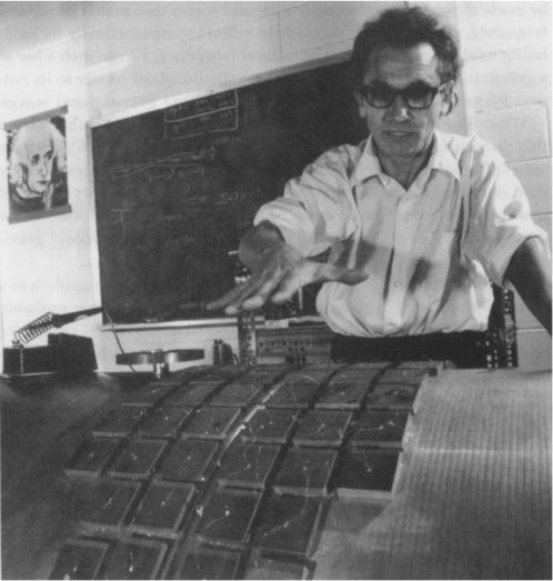
10.4 Joseph Weber, demonstrating the piezoelectric crystals glued around the middle of his aluminum bar; ca. 1973. Gravitational waves should drive the bar’s end-to-end vibrations, and those vibrations should squeeze the crystals in and out so they produce oscillating voltages that are detected electronically. [Photo by James P. Blair, courtesy the National Geographic Society.]
Weber’s sensor was based on the piezoelectric effect, in which certain kinds of materials (certain crystals and ceramics), when squeezed slightly, develop electric voltages from one end to the other. Weber would have liked to make his bar from such a material, but these materials were far too expensive, so he did the next best thing: He made his bar from aluminum, and he then glued piezoelectric crystals around the bar’s middle (Figure 10.4). As the bar vibrated, its surface squeezed and stretched the crystals, each crystal developed an oscillating voltage, and Weber strung the crystals together one after another in an electric circuit so their tiny oscillating voltages would add up to a large enough voltage for electronic detection, even when the bar’s vibrations were only one-tenth the diameter of the nucleus of an atom.
In the early 1960s, Weber was a lonely figure, the only experimental physicist in the world seeking gravitational waves. With his bitter aftertaste of laser competition, he enjoyed the loneliness. However, in the early 1970s, his impressive sensitivities and evidence that he might actually be detecting waves (which, in retrospect, I am convinced he was not) attracted dozens of other experimenters, and by the 1980s more than a hundred talented experimenters were engaged in a competition with him to make gravitational-wave astronomy a reality.
I first met Weber on a hillside opposite Mont Blanc in the French Alps, in the summer of 1963, four years after he embarked on his project to detect gravitational waves. I was a graduate student, just beginning research in relativity, and along with thirty-five other students from around the world I had come to the Alps for an intensive two-month summer school focusing solely on Einstein’s general relativistic laws of gravity. Our teachers were the world’s greatest relativity experts—John Wheeler, Roger Penrose, Charles Misner, Bryce DeWitt, Joseph Weber, and others—and we learned from them in lectures and private conversations, with the glistening snows of the Aguille de Midi and Mont Blanc towering high in the sky above us, belled cows grazing in brilliant green pastures around us, and the picturesque village of Les Houches several hundred meters below us, at the foot of our school’s hillside.
In this glorious setting, Weber lectured about gravitational waves and his project to detect them, and I listened, fascinated. Between lectures Weber and I conversed about physics, life, and mountain climbing, and I came to regard him as a kindred soul. We were both loners; neither of us enjoyed intense competition or vigorous intellectual give-and-take. We both preferred to wrestle with a problem on our own, seeking advice and ideas occasionally from friends, but not being buffeted by others who were trying to beat us to a new insight or discovery.
Over the next decade, as research on black holes heated up and entered its golden age (Chapter 7 ), I began to find black-hole research distasteful—too much intensity, too much competition, too much rough-and-tumble. So I cast about for another area of research, one with more elbow room, into which I could put most of my effort while still working on black holes and other things part time. Inspired by Weber, I chose gravitational waves.
Like Weber, I saw gravitational waves as an infant research field with a bright future. By entering the field in its infancy, I could have the fun of helping mold it, I could lay foundations on which others later would build, and I could do so without others breathing down my neck, since most other relativity theorists were then focusing on black holes.
For Weber, the foundations to be laid were experimental: the invention, construction, and continual improvement of detectors. For me, they were theoretical: try to understand what Einstein’s gravitational laws have to say about how gravitational waves are produced, how they push back on their sources as they depart, and how they propagate; try to figure out which kinds of astronomical objects will produce the Universe’s strongest waves, how strong their waves will be, and with what frequencies they will oscillate; invent mathematical tools for computing the details of the encoded symphonies produced by these objects, so when Weber and others ultimately detect the waves, theory and experiment can be compared.
I n 1969 I spent six weeks in Moscow, at Zel’dovich’s invitation. One day Zel’dovich took time out from bombarding me and others with new ideas (Chapters 7 and 12 ), and drove me over to Moscow University to introduce me to a young experimental physicist, Vladimir Braginsky. Braginsky, stimulated by Weber, had been working for several years to develop techniques for gravitational-wave detection; he was the first experimenter after Weber to enter the field. He was also in the midst of other- fascinating experiments: a search for quarks (a fundamental building block of protons and neutrons), and an experiment to test Einstein’s assertion that all objects, no matter what their composition, fall with the same acceleration in a gravitational field (an assertion that underlies Einstein’s description of gravity as spacetime curvature).
I was impressed. Braginsky was clever, deep, and had excellent taste in physics; and he was warm and forthright, as easy to talk to about politics as about science. We quickly became close friends and learned to respect each other’s world views. For me, a liberal Democrat in the American spectrum, the freedom of the individual was paramount over all other considerations. No government should have the right to dictate how one lives one’s life. For Braginsky, a nondoctrinaire Communist, the responsibility of the individual to society was paramount. We are our brothers’ keepers, and well we should be in a world where evil people like Joseph Stalin can gain control if we are not vigilant.
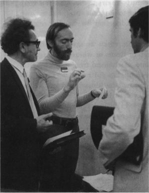
Joseph Weber, Kip Thorne, and Tony Tyson at a conference on gravitational radiation in Warsaw, Poland, September 1973. [photo by Marek Holzman, courtesy Andrzej Trautman;]
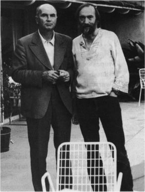
Vladimir Braginsky and Kip Thorne, in Pasadena, California, October 1984. [courtesy Valentin N. Rudenko.]
Braginsky had foresight that nobody else possessed. During our 1969 meeting, and then again in 1971 and 1972, he warned me that the bars being used to search for gravitational waves have a fundamental, ultimate limitation. That limitation, he told me, comes from the laws of quantum mechanics. Although we normally think of quantum mechanics as governing tiny objects such as electrons, atoms, and molecules, if we make sufficiently precise measurements on the vibrations of a one-ton bar, we should see those vibrations also behave quantum mechanically, and their quantum mechanical behavior will ultimately cause problems for gravitational-wave detection. Braginsky had convinced himself of this by calculating the ultimate performance of Weber’s piezoelectric crystals and of several other kinds of sensors that one might use to measure a bar’s vibrations.
I didn’t understand what Braginsky was talking about; I didn’t understand his reasoning, I didn’t understand his conclusion, I didn’t understand its importance, and I didn’t pay much attention. Other things he was teaching me seemed much more important: From him I was learning how to think about experiments, how to design experimental apparatus, how to predict the noise that will plague the apparatus, and how to suppress the noise so the apparatus will succeed in its task—and from me, Braginsky was learning how to think about Einstein’s laws of gravity, how to identify their predictions. We were rapidly becoming a team, each bringing to our joint enterprise his own expertise; and over the next two decades, together we would have great fun and make a few discoveries.
Each year in the early and mid-1970s, when we saw each other in Moscow or Pasadena or Copenhagen or Rome or wherever, Braginsky repeated his warning about quantum mechanical trouble for gravitational- wave detectors, and each year I again did not understand. His warning was somewhat muddled because he himself did not understand fully what was going on. However, in 1976, after Braginsky, and independently Robin Giffard at Stanford University, managed to make the warning more clear, I suddenly understood. The warning was serious, I finally realized; the ultimate sensitivity of a bar detector is severely limited by the uncertainty principle.
T he uncertainty principle is a fundamental feature of the laws of quantum mechanics. It says that, if you make a highly accurate measurement of the position of an object, then in the process of your measurement you will necessarily kick the object, thereby perturbing the object’s velocity in a random, unpredictable way. The more accurate your position measurement is, the more strongly and unpredictably you must perturb the object’s velocity. No matter how clever you are in designing your measurement, you cannot circumvent this innate uncertainty. (See Box 10.2.)
Box 10.2
The Uncertainty Principle and Wave/Particle Duality
The uncertainty principle is intimately related to wave/particle duality (Box 4.1)—that is, to the propensity of particles to act sometimes like waves and sometimes like particles.
If you measure the position of a particle (or any other object, for example, the end of a bar) and learn that it is somewhere inside some error box, then regardless of what the particle’s wave might have looked like before the measurement, during the measurement the measuring apparatus will “kick” the wave and thereby confine it inside the error box’s interior. The wave, thereby, will acquire a confined form something like the following:
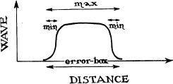
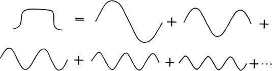
Such a confined wave contains many different wavelengths, ranging from the size of the box itself (marked max above) to the tiny size of the corners at which the wave begins and ends (marked min). More specifically, the confined wave can be constructed by adding together, that is, superimposing, the following oscillatory waves, which have wavelengths ranging from max down to min:
Now, recall that the shorter the wavelength of the wave’s oscillations, the larger the energy of the particle, and thus also the larger the particle’s velocity. Since the measurement has given the wave a range of wavelengths, the particle’s energy and velocity might now be anywhere in the corresponding ranges; in other words, its energy and velocity are uncertain.
To recapitulate, the measurement confined the particle’s wave to the error box (first diagram above); this made the wave consist of a range of wavelengths (second diagram); that range of wavelengths corresponds to a range of energy and velocity; and the velocity is therefore uncertain. No matter how hard you try, you cannot avoid producing this velocity uncertainty when you measure the particle’s position. Moreover, when this chain of reasoning is examined in greater depth, it predicts that the more accurate your measurement, that is, the smaller your error box, the larger the ranges of wavelengths and velocity, and thus the larger the uncertainty in the particle’s velocity.
The uncertainty principle governs not only measurements of microscopic objects such as electrons, atoms, and molecules; it also governs measurements of large objects. However, because a large object has large inertia, a measurement’s kick will perturb its velocity only slightly. (The velocity perturbation will be inversely proportional to the object’s mass.)
The uncertainty principle, when applied to a gravitational-wave detector, says that the more accurately a sensor measures the position of the end or side of a vibrating bar, the more strongly and randomly the measurement must kick the bar.
For an inaccurate sensor, the kick can be tiny and unimportant, but because the sensor was inaccurate, you do not know very well the amplitude of the bar’s vibrations and thus cannot monitor weak gravitational waves.
For an extremely accurate sensor, the kick is so enormous that it strongly changes the bar’s vibrations. These large, unknowable changes thus mask the effects of any gravitational wave you might try to detect.
Somewhere between these two extremes there is an optimal accuracy for the sensor: an accuracy neither so poor that you learn little nor so great that the unknowable kick is strong. At that optimal accuracy, which is now called Braginsky’s standard quantum limit, the effect of the kick is just barely as debilitating as the errors made by the sensor. No sensor can monitor the bar’s vibrations more accurately than this standard quantum limit. How small is this limit? For a 2-meter-long, 1-ton bar, it is about 100,000 times smaller than the nucleus of an atom.
In the 1960s, nobody seriously contemplated the need for such accurate measurements, because nobody understood very clearly just how weak should be the gravitational waves from black holes and other astronomical bodies. But by the mid-1970s, spurred on by Weber’s experimental project, I and other theorists had begun to figure out how strong the strongest waves were likely to be. Roughly 10 −21 was the answer, and this meant the waves would make a 2-meter bar vibrate with an amplitude of only 10 −21 × (2 meters), or about a millionth the diameter of the nucleus of an atom. If these estimates were correct (and we knew they were highly uncertain), then the gravitational-wave signal would be ten times smaller than Braginsky’s standard quantum limit, and therefore could not possibly be detected using a bar and any known kind of sensor.
Though this was extremely worrisome, all was not lost. Braginsky’s deep intuition told him that, if experimenters were especially clever, they ought to be able to circumvent his standard quantum limit. There ought to be a new way to design a sensor, he argued, so that its unknowable and unavoidable kick does not hide the influence of the gravitational waves on the bar. To such a sensor Braginsky gave the name quantum nondemolition 3 ; “quantum” because the sensor’s kick is demanded by the laws of quantum mechanics, “nondemolition” because the sensor would be so configured that the kick would not demolish the thing you are trying to measure, the influence of the waves on the bar. Braginsky did not have a workable design for a quantum nondemolition sensor, but his intuition told him that such a sensor should be possible.
This time I listened, carefully; and over the next two years I and my group at Caltech and Braginsky and his group in Moscow both struggled, on and off, to devise a quantum nondemolition sensor.
We both found the answer simultaneously in the autumn of 1977—but by very different routes. I remember vividly my excitement when the idea occurred to Carlton Caves and me 4 in an intense discussion over lunch at the Greasy (Caltech’s student cafeteria). And I recall the bittersweet taste of learning that Braginsky, Yuri Vorontsov, and Farhid Khalili had had a significant piece of the same idea in Moscow at essentially the same time—bitter because I get great satisfaction from being the first to discover something new; sweet because I am so fond of Braginsky and thus get pleasure from sharing discoveries with him.
Our full quantum nondemolition idea is rather abstract and permits a wide variety of sensor designs for circumventing Braginsky’s standard quantum limit. The idea’s abstractness, however, makes it difficult to explain, so here I shall describe just one (not very practical) example of a quantum nondemolition sensor. 5 This example has been called, by Braginsky, a stroboscopic sensor.
A stroboscopic sensor relies on a special property of a bar’s vibrations: If the bar is given a very sharp, unknown kick, its amplitude of vibration will change, but no matter what that amplitude change is, precisely one period of oscillation after the kick the bar’s vibrating end will return to the same position as it had at the moment of the kick (black dots in Figure 10.5). At least this is true if a gravitational wave (or some other force) has not squeezed or stretched the bar in the meantime. If a wave (or other force) has squeezed the bar in the meantime, then the bar’s position one period later will be changed.
To detect the wave, then, one should build a sensor that makes stroboscopic measurements of the bar’s vibrating ends, a sensor that measures the position of the bar’s ends quickly once each period of vibration. Such a sensor will kick the bar in each measurement, but the kicks will not change the position of the bar’s ends at the times of subsequent measurements. If the position is found to have changed, then a gravitational wave (or some other force) must have squeezed the bar.
A lthough quantum nondemolition sensors solved the problem of Braginsky’s standard quantum limit, by the mid-1980s I had become rather pessimistic about the prospects for bar detectors to bring gravitational- wave astronomy to fruition. My pessimism had two causes.
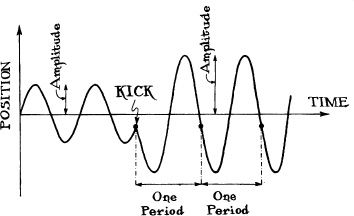
10.5 The principle underlying a stroboscopic quantum nondemolition measurement. Plotted vertically is the position of the end of a vibrating bar; plotted horizontally is time. If a quick, highly precise measurement of the position is made at the time marked KICK, the sensor that makes the measurement will give the bar a sudden, unknowable kick, thereby changing the bar’s amplitude of vibration in an unknown way. However, there will be no change of the position of the bar’s end precisely one period after the kick, or two periods, or three periods. Those positions will be the same as at the time of the kick and will be completely independent of the kick.
First, although the bars built by Weber, by Braginsky, and by others had achieved far better sensitivities than anyone had dreamed possible in the 1950s, they were still only able to detect with confidence waves of strength 10 −17 or larger. This was 10,000 times too poor for success, if I and others had correctly estimated the strengths of the waves arriving at Earth. This by itself was not serious, since the march of technology has often produced 10,000-fold improvements in instruments over times of twenty years or less. [One example was the angular resolution of the best radio telescopes, which improved from tens of degrees in the mid-1940s to a few arc seconds in the mid-1960s (Chapter 9 ). Another was the sensitivity of astronomical X-ray detectors, which improved by a factor of 10 10 between 1958 and 1978, that is, at an average rate of 10,000 every eight years (Chapter 8 ).] However, the rate of improvement of the bars was so slow, and projections of the future technology and techniques were so modest, that there seemed no reasonable way for a 10,000-fold improvement to be made in the foreseeable future. Success, thus, would likely hinge on the waves being stronger than the 10 −21 estimates—a real possibility, but not one that anybody was happy to rely on.
Second, even if the bars did succeed in detecting gravitational waves, they would have enormous difficulty in decoding the waves’ symphonic signals, and in fact would probably fail. The reason was simple: Just as a tuning fork or wine glass responds sympathetically only to a sound whose frequency is close to its natural frequency, so a bar would respond only to gravitational waves whose frequency is near the bar’s natural frequency; in technical language, the bar detector has a narrow bandwidth (the bandwidth being the band of frequencies to which it responds). But the waves’ symphonic information should typically be encoded in a very wide band of frequencies. To extract the waves’ information, then, would require a “xylophone” of many bars, each covering a different, tiny portion of the signal’s frequencies. How many bars in the xylophone? For the types of bars then being planned and constructed, several thousand—far too many to be practical. In principle it would be possible to widen the bars’ bandwidths and thereby manage with, say, a dozen bars, but to do so would require major technical advances beyond those for reaching a sensitivity of 10 −21 .
Although I did not say much in public in the 1980s about my pessimistic outlook, in private I regarded it as tragic because of the great effort that Weber, Braginsky, and my other friends and colleagues had put into bars, and also because I had become convinced that gravitational radiation has the potential to produce a revolution in our knowledge of the Universe.
LIGO
T o understand the revolution that the detection and deciphering of gravitational waves might bring, let us recall the details of a previous revolution: the one created by the development of X-ray and radio telescopes (Chapters 8 and 9 ).
In the 1930s, before the advent of radio astronomy and X-ray astronomy, our knowledge of the Universe came almost entirely from light. Light showed it to be a serene and quiescent Universe, a Universe dominated by stars and planets that wheel smoothly in their orbits, shining steadily and requiring millions or billions of years to change in discernible ways.
This tranquil view of the Universe was shattered, in the 1950s, 1960s, and 1970s, when radio-wave and X-ray observations showed us our Universe’s violent side: jets ejected from galactic nuclei, quasars with fluctuating luminosities far brighter than our galaxy, pulsars with intense beams shining off their surfaces and rotating at high speeds. The brightest objects seen by optical telescopes were the Sun, the planets, and a few nearby, quiescent stars. The brightest objects seen by radio telescopes were violent explosions in the cores of distant galaxies, powered (presumably) by gigantic black holes. The brightest objects seen by X-ray telescopes were small black holes and neutron stars accreting hot gas from binary companions.
What was it about radio waves and X-rays that enabled them to create such a spectacular revolution? The key was the fact that they brought us very different kinds of information than is brought by light: Light, with its wavelength of a half micron, was emitted primarily by hot atoms residing in the atmospheres of stars and planets, and it thus taught us about those atmospheres. The radio waves, with their 10million- fold greater wavelengths, were emitted primarily by near-light-speed electrons spiraling in magnetic fields, and they thus taught us about the magnetized jets shooting out of galactic nuclei, about the gigantic, magnetized intergalactic lobes that the jets feed, and about the magnetized beams of pulsars. The X-rays, with their thousand-fold shorter wavelengths than light, were produced mostly by high-speed electrons in ultra-hot gas accreting onto black holes and neutron stars, and they thus taught us directly about the accreting gas and indirectly about the holes and neutron stars.
The differences between light, on the one hand, and radio waves and X-rays, on the other, are pale compared to the differences between the electromagnetic waves (light, radio, infrared, ultraviolet, X-ray, and gamma ray) of modern astronomy and gravitational waves. Correspondingly, gravitational waves might revolutionize our understanding of the Universe even more than did radio waves and X-rays. Among the differences between electromagnetic waves and gravitational waves, and their consequences, are these 6 :
• The gravitational waves should be emitted most strongly by large-scale, coherent vibrations of spacetime curvature (for example, the collision and coalescence of two black holes) and by large-scale, coherent motions of huge amounts of matter (for example, the implosion of the core of a star that triggers a supernova, or the inspiral and merger of two neutron stars that are orbiting each other). Therefore, gravitational waves should show us the motions of huge curvatures and huge masses. By contrast, cosmic electromagnetic waves are usually emitted individually and separately by enormous numbers of individual and separate atoms or electrons; and these individual electromagnetic waves, each oscillating in a slightly different manner, then superimpose on each other to produce the total wave that an astronomer measures. As a result, from electromagnetic waves we learn primarily about the temperature, density, and magnetic fields experienced by the emitting atoms and electrons.
• Gravitational waves are emitted most strongly in regions of space where gravity is so intense that Newton’s description fails and must be replaced by Einstein’s, and where huge amounts of matter or spacetime curvature move or vibrate or swirl at near the speed of light. Examples are the big bang origin of the Universe, the collisions of black holes, and the pulsations of newborn neutron stars at the centers of supernova explosions. Since these strong-gravity regions are typically surrounded by thick layers of matter that absorb electromagnetic waves (but do not absorb gravitational waves), the strong-gravity regions cannot send us electromagnetic waves. The electromagnetic waves seen by astronomers come, by contrast, almost entirely from weak-gravity, low-velocity regions; for example, the surfaces of stars and supernovae.
These differences suggest that the objects whose symphonies we might study with gravitational-wave detectors will be largely invisible in light, radio waves, and X-rays; and the objects that astronomers now study in light, radio waves, and X-rays will be largely invisible in gravitational waves. The gravitational Universe should thus look extremely different from the electromagnetic Universe; from gravitational waves we should learn things that we will never learn electromagnetically. This is why gravitational waves are likely to revolutionize our understanding of the Universe.
It might be argued that our present electromagnetically based understanding of the Universe is so complete compared with the optically based understanding of the 1930s that a gravitational-wave revolution will be far less spectacular than was the radio-wave/X-ray revolution. This seems to me unlikely. I am painfully aware of our lack of understanding when I contemplate the sorry state of present estimates of the gravitational waves bathing the Earth. For each type of gravitational-wave source that has been thought about, with the exception of binary stars and their coalescences, either the strength of the source’s waves for a given distance from Earth is uncertain by several factors of 10, or the rate of occurrence of that type of source (and thus also the distance to the nearest one) is uncertain by several factors of 10, or the very existence of the source is uncertain.
These uncertainties cause great frustration in the planning and design of gravitational-wave detectors. That is the downside. The upside is the fact that, if and when gravitational waves are ultimately detected and studied, we may be rewarded with major surprises.
I n 1976 I had not yet become pessimistic about bar detectors. On the contrary, I was highly optimistic. The first generation of bar detectors had recently reached fruition and had operated with a sensitivity that was remarkable compared to what one might have expected; Braginsky and others had invented a number of clever and promising ideas for huge future improvements; and I and others were just beginning to realize that gravitational waves might revolutionize our understanding of the Universe.
My enthusiasm and optimism drove me, one evening in November 1976, to wander the streets of Pasadena until late into the night, struggling with myself over whether to propose that Caltech create a project to detect gravitational waves. The arguments in favor were obvious: for science in general, the enormous intellectual payoff if the project succeeded; for Caltech, the opportunity to get in on the ground floor of an exciting new field; for me, the possibility to have a team of experimenters at my home institution with whom to interact, instead of relying primarily on Braginsky and his team on the other side of the world, and the possibility to play a more central role than I could commuting to Moscow (and thereby have more fun). The argument against was also obvious: The project would be risky; to succeed, it would require large resources from Caltech and the D.S. National Science Foundation and enormous time and energy from me and others; and after all that investment, it might fail. It was much more risky than Caltech’s entry into radio astronomy twenty-three years earlier (Chapter 9 ).
After many hours of introspection, the lure of the payoffs won me over. And after several months studying the risks and payoffs, Caltech’s physics and astronomy faculty and administration unanimously approved my proposal—subject to two conditions. We would have to find an outstanding experimental physicist to lead the project, and the project would have to be large enough and strong enough to have a good chance of success. This meant, we believed, much larger and stronger than Weber’s effort at the University of Maryland or Braginsky’s effort in Moscow or any of the other gravitational-wave efforts then under way.
The first step was finding a leader. I flew to Moscow to ask Braginsky’s advice and feel him out about taking the post. My feeler tore him every which way. He was torn between the far better technology he would have in America and the greater craftsmanship of the technicians in Moscow (for example, intricate glassblowing was almost a lost art in America, but not in Moscow). He was torn between the need to build a project from scratch in America and the crazy impediments that the inefficient, bureaucracy-bound Soviet system kept putting in the way of his project in Moscow. He was torn between loyalty to his native land and disgust with his native land, and between his feelings that life in America is barbaric because of the way we treat our poor and our lack of medical care for everyone and his feelings that life in Moscow is miserable because of the power of incompetent officials. He was torn between the freedom and wealth of America and fear of KGB retribution against family and friends and perhaps even himself if he “defected.” In the end he said no, and recommended instead Ronald Drever of Glasgow University.
Others I consulted were also enthusiastic about Drever. Like Braginsky, he was highly creative, inventive, and tenacious—traits that would be essential for success of the project. The Caltech faculty and administration gathered all the information they could about Drever and other possible leaders, selected Drever, and invited him to join the Caltech faculty and initiate the project. Drever, like Braginsky, was torn, but in the end he said yes. We were off and running.
I had presumed, when proposing the project, that like Weber and Braginsky, Caltech would focus on building bar detectors. Fortunately (in retrospect) Drever insisted on a radically different direction. In Glasgow he had worked with bar detectors for five years, and he could see their limitations. Much more promising, he thought, were interferometric gravitational-wave detectors (interferometers for short—though they are radically different from the radio interferometers of Chapter 9 ).
Interferometers for gravitational-wave detection had first been conceived of in primitive form in 1962 by two Russian friends of Braginsky’s, Mikhail Gertsenshtein and V.I. Pustovoit, and independently in 1964 by Joseph Weber. Unaware of these early ideas, Rainer Weiss devised a more mature variant of an interferometric detector in 1969, and then he and his MIT group went on to design and build one in the early 1970s, as did Robert Forward and colleagues at Hughes Research Laboratories in Malibu, California. Forward’s detector was the first to operate successfully. By the late 1970s, these interferometric detectors had become a serious alternative to bars, and Drever had added his own clever twists to their design.
F igure 10.6 shows the basic idea behind an interferometric gravitational-wave detector. Three masses hang by wires from overhead supports at the corner and ends of an “L” (Figure 10.6a). When the first crest of a gravitational wave enters the laboratory from overhead or underfoot, its tidal forces should stretch the masses apart along one arm of the “L” while squeezing them together along the other arm. The result will be an increase in the length L 1 of the first arm (that is, in the distance between the arm’s two masses) and a decrease in the length L 2 of the second arm, When the wave’s first crest has passed and its first trough arrives, the directions of stretch and squeeze will be changed: L 1 will decrease and L 2 will increase. By monitoring the arm-length difference, L 1 – L 2 , one can seek gravitational waves.
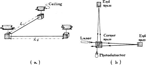
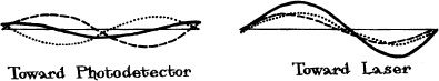
10.6 A laser interferometric gravitational-wave detector. This instrument is very similar to the one used by Michelson and Morley in 1887 to search for motion of the Earth through the aether ( Chapter 1 ). See the text for a detailed explanation.
The difference L 1 – L 2 is monitored using interferometry (Figure 10.6b and Box 10.3). A laser beam shines onto a beam splitter that rides on the corner mass. The beam splitter reflects half of the beam and transmits half, and thereby splits the beam in two. The two beams go down the two arms of the interferometer and bounce off mirrors that ride on the arms’ end masses, and then return to the beam splitter. The splitter half-transmits and half-reflects each of the beams, so part of each beam’s light is combined with part from the other and goes back toward the laser, and the other parts of the two beams are combined and go toward the photodetector. When no gravitational wave is present, the contributions from the two arms interfere in such a way (Box 10.3) that all the net light goes back toward the laser and none toward the photodetector. If a gravitational wave slightly changes L 1 - L 2 , the two beams will then travel slightly different distances in their two arms and will interfere slightly differently—a tiny amount of their combined light will now go into the photodetector. By monitoring the amount of light reaching the photodetector, one can monitor the arm-length difference L 1 - L 2 , and thereby monitor gravitational waves.
Box 10.3
Interference and Interferometry
Whenever two or more waves propagate through the same region of space, they superimpose on each other “linearly” (Box 10.1); that is, they add. For example, the following dotted wave and dashed wave superimpose to produce the heavy solid wave:
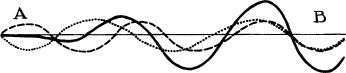
Notice that at locations such as A where a trough of one wave (dotted) superimposes on a crest of the other (dashed), the waves cancel, at least in part, to produce a vanishing or weak total wave (solid); and at locations such as B where two troughs superimpose or two crests superimpose, the waves reinforce each other. One says that the waves are interfering with each other, destructively in the first case and constructively in the second. Such superimposing and interference occurs in all types of waves—ocean waves, radio waves, light waves, gravitational waves—and such interference is central to the operation of radio interferometers ( Chapter 9 ) and interferometric detectors for gravitational waves.
In the interferometric detector of Figure 10.6b, the beam splitter superimposes half the light wave from one arm on half from the other and sends them toward the laser, and it superimposes the other halves and sends them toward the photodetector. When no gravitational wave or other force has moved the masses and their mirrors, the superimposed light waves have the following forms, where the dashed curve shows the wave from arm 1, the dotted curve the wave from arm 2, and the solid curve the superimposed, total wave:
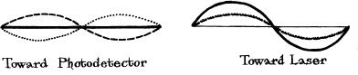
Toward the photodetector, the waves interfere perfectly destructively, so the total, superimposed wave vanishes, which means that the photodetector sees no light at all. When a gravitational wave or other force has lengthened op.e arm slightly and shortened the other, then the beam from the one arm arrives at the beam splitter with a slight delay relative to the other, and the superimposed waves therefore look like this:
The destructive interference in the photodetector’s direction is no longer perfect; the photodetector receives some light. The amount it receives is proportional to the arm length difference, L 1 – L 2 which in turn is proportional to the gravitational-wave signal.
I t is interesting to compare a bar detector with an interferometer. The bar detector uses the vibrations of a single, solid cylinder to monitor the tidal forces of a gravitational wave. The interferometric detector uses the relative motions of masses hung from wires to monitor the tidal forces.
The bar detector uses an electrical sensor (for example, piezoelectric crystals squeezed by the bar) to monitor the bar’s wave-induced vibrations. The interferometric detector uses interfering light beams to monitor its masses’ wave-induced motions.
The bar responds sympathetically only to gravitational waves over a narrow frequency band, and therefore, decoding the waves’ symphony would require a xylophone of many bars. The interferometer’s masses wiggle back and forth in response to waves of all frequencies higher than about one cycle per second, 7 and tllerefore the interferometer has a wide bandwidth; three or four interferometers are sufficient to fully decode the symphony.
By making the interferometer’s arms a thousand times longer than the bar (a few kilometers rather than a few meters), one can make the waves’ tidal forces a thousand times bigger and thus improve the sensitivity of the instrument a thousand-fold. 8 The bar, by contrast, cannot be lengthened much. A kilometer-Iong bar would have a natural frequency less than one cycle per second and thus would not operate at the frequencies where we think the most interesting sources lie. Moreover, at such a low frequency, one must launch the bar into space to isolate it from vibrations of the ground and from the fluctuating gravity of the Earth’s atmosphere. Putting such a bar in space would be ridiculously expensIve.
Because it is a thousand times longer than the bar, the interferometer is a thousand times more immune to the “kick” produced by the measurement process. This immunity means that the interferometer does not need to circumvent the kick with the aid of a (difficult to construct) quantum nondemolition sensor. The bar, by contrast, can detect the expected waves only if it employs quantum nondemolition.
If the interferometer has such great advantages over the bar (far larger bandwidth and far larger potential sensitivity), then why didn’t Braginsky, Weber, and others build interferometers instead of bars? When I asked Braginsky in the mid-1970s, he replied that bar detectors are simple, while interferometers are horrendously complex. A small, intimate team like his in Moscow had a reasonable chance of making bar detectors work well enough to discover gravitational waves. However, to construct, debug, and operate interferometric detectors success fully would require a huge team and large amounts of money—and Braginsky doubted whether, even with such a team and such money, so complex a detector could succeed.
Ten years later, as the painful evidence mounted that bars would have great difficulty reaching 10 −21 sensitivity, Braginsky visited Caltech and was impressed with the progress that Drever’s team had achieved with interferometers. Interferometers, he concluded, will probably succeed after all. But the huge team and large money required for success were not to his taste; so upon returning to Moscow, he redirected most of his own team’s efforts away from gravitational-wave detection. (Elsewhere in the world bars have continued to be developed, which is fortunate; they are cheap compared to interferometers, for now they are more sensitive, and in the long run they might play special roles at high gravity-wave frequencies.)
W herein lies the complexity of interferometric detectors? After all, the basic idea, as described in Figure 10.6, looks reasonably simple.
In fact, Figure 10.6 is a gross oversimplification because it ignores an enormous number of pitfalls. The tricks required to avoid these pitfalls make an interferometer into a very complex instrument. For example, the laser beam must point in precisely the right direction and have precisely the right shape and wavelength to fit into the interferometer perfectly; and its wavelength and intensity must not fluctuate. After the beam is split in half, the two beams must bounce back and forth in the two arms not just once as in Figure 10.6, but many times, so as to increase their sensitivity to the wiggling masses’ motions, and after these many bounces, they must meet each other perfectly back at the beam splitter. Each mass must be continually controlled so its mirrors point in precisely the right directions and do not swing as a result of vibrations of the floor, and this must be done without masking the mass’s gravitational-wave-induced wiggles. To achieve perfection in all these ways, and in many many more, requires continuously monitoring many different pieces of the interferometer and its light beams, and continuously applying feedback forces to keep them perfect.
One gets some impression of these complications from a photograph (Figure 10.7) of a 40-meter-Iong prototype interferometric detector that Drever’s team has built at Caltech—a prototype which itself is far simpler than the full-scale, several-kilometer-Iong interferometers that are required for success.
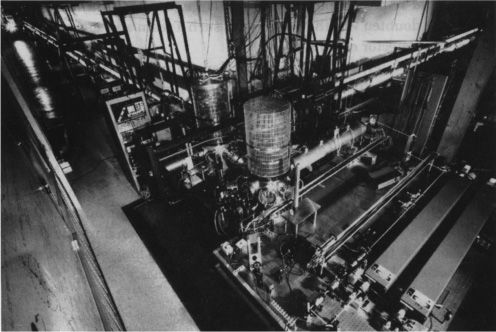
10.7 The Caltech 40-meter interferometric prototype gravitational-wave detector, ca. 1989. The table in front and the front caged vacuum chamber hold lasers and devices to prepare the laser light for entry into the interferometer. The central mass resides in the second caged vacuum chamber—the chamber above which a dangling rope can be seen faintly. The end masses are 40 meters away, down the two corridors. The two arms’ laser beams shine down the larger of the two vacuum pipes that extend the lengths of the corridors . [Courtesy LIGO Project, California Institute of Technology.]
D uring the early 1980s four teams of experimental physicists struggled to develop tools and techniques for interferometric detectors: Drever’s Caltech team, the team he had founded at Glasgow (now led by James Hough), Rainer Weiss’s team at MIT, and a team founded by Hans Billing at the Max Planck Institut in Munich, Germany. The teams were small and intimate, and they worked more or less independently, 9 pursuing their own approaches to the design of interferometric detectors. Within each team the individual scientists had free rein to invent new ideas and pursue them as they wished and for as long as they wished; coordination was very loose. This is just the kind of culture that inventive scientists love and thrive on, the culture that Braginsky craves, a culture in which loners like me are happiest. But it is not a culture capable of designing, constructing, debugging, and operating large, complex scientific instruments like the several-kilometer-long interferometers required for success.
To design in detail the many complex pieces of such interferometers, to make them all fit together and work together properly, and to keep costs under control and bring the interferometers to completion within a reasonable time require a different culture: a culture of tight coordination, with subgroups of each team focusing on well-defined tasks and a single director making decisions about what tasks will be done when and by whom.
The road from freewheeling independence to tight coordination is a painful one. The world’s biology community is traveling that road, with cries of anguish along the way, as it moves toward sequencing the human genome. And we gravitational-wave physicists have been traveling that road since 1984, with no less pain and anguish. I am confident, however, that the excitement, pleasure, and scientific payoff of detecting the waves and deciphering their symphonies will one day make the pain and anguish fade in our memories.
The first sharp turn on our painful road was a 1984 shotgun marriage between the Caltech and MIT teams—each of which by then had about eight members. Richard Isaacson of the D.S. National Science Foundation (NSF) held the shotgun and demanded, as the price of the taxpayers’ financial support, a tight marriage in which Caltech and MIT scientists jointly developed the interferometers. Drever (resisting like mad) and Weiss (willingly accepting the inevitable) said their vows, and I became the marriage counselor, the man with the task of forging consensus when Drever pulled in one direction and Weiss in another. It was a rocky marriage, emotionally draining for all; but gradually we began to work together.
The second sharp turn came in November 1986. A committee of eminent physicists—experts in all the technologies we need and experts in the organization and management of large scientific projects—spent an entire week with us, scrutinizing our progress and plans, and then reported to NSF. Our progress got high marks, our plans got high marks, and our prospects for success—for detecting waves and deciphering their symphonies—were rated as high. But our culture was rated as awful; we were still immersed in the loosely knit, freewheeling culture of our birth, and we could never succeed that way, NSF was told. Replace the Drever—Weiss—Thorne troika by a single director, the committee insisted—a director who can mold talented individualists into a tightly knit and effective team and can organize the project and make firm, wise decisions at every major juncture.
Out came the shotgun again. If you want your project to continue, NSF’s Isaacson told us, you must find that director and learn to work with him like a football team works with a great coach or an orchestra with a great conductor.
We were lucky. In the midst of our search, Robbie Vogt got fired.
Vogt, a brilliant, strong-willed experimental physicist, had directed projects to construct and operate scientific instruments on spacecraft, had directed the construction of a huge millimeter-wavelength astronomical interferometer, and had reorganized the scientific research environment of NASA’s Jet Propulsion Laboratory (which carries out most of the American planetary exploration program)—and he then had become Caltech’s provost. As provost, though remarkably effective, Vogt battled vigorously with Caltech’s president, Marvin Goldberger, over how to run Caltech—and after several years of battle, Goldberger fired him. Vogt was not temperamentally suited to working under others when he disagreed profoundly with their judgments; but on top, he was superb. He was just the director, the conductor, the coach that we needed. If anybody could mold us into a tightly knit team, he could.
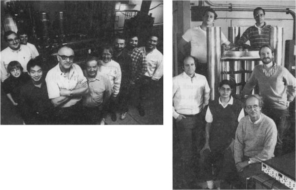
A portion of the Caltech/MIT team of LIGO scientists in late 1991. Left: Some Caltech members of the team, counterclockwise from upper left: Aaron Gillespie, Fred Raab, Maggie Taylor, Seiji Kawamura, Robbie Vogt, Ronald Drever, Lisa Sievers, Alex Abramovici, Bob Spero, Mike Zucker. Right: Some MIT members of the team,. counterclockwise from upper left: Joe Kovalik, Yaron Hefetz, Nergis Mavalvala, Rainer Weiss, David Schumaker, Joe Giaime. [Left: courtesy Ken Rogers/ Black Star; right: courtesy Erik L. Simmons.
“It will be painful working with Robbie,” a former member of his millimeter team told us. “You will emerge bruised and scarred, but it will be worth it. Your project will succeed.”
For several months Drever, Weiss, I, and others pleaded with Vogt to take the directorship. He finally accepted; and, as promised, six years later our Caltech/MIT team is bruised and scarred, but effective, powerful, tightly knit, and growing rapidly toward the critical size (about fifty scientists and engineers) required for success. Success, however, will not depend on us alone. Under Vogt’s plan important inputs to our core effort will come from other scientists 10 who, by being only loosely associated with us, can maintain the individualistic, free-wheeling style that we have left behind.
A key to success in our endeavor will be the construction and operation of a national scientific facility called the Laser Interferometer Gravitational-Wave Observatory, or LIGO. The LIGO will consist of two L-shaped vacuum systems, one near Hanford, Washington, and the other near Livingston, Louisiana, in which physicists will develop and operate many successive generations of ever-improving interferometers; see Figure 10.8.
Why two facilities instead of one? Because Earth-bound gravitational-wave detectors always have ill-understood noise that simulates gravitational-wave bursts; for example, the wire that suspends a mass can creak slightly for no apparent reason, thereby shaking the mass and simulating the tidal force of a wave. However, such noise almost never happens simultaneously in two independent detectors, far apart. Thus, to be sure that an apparent signal is due to gravitational waves rather than noise, one must verify that it occurs in two such detectors. With only one detector, gravitational waves cannot be detected and monitored.
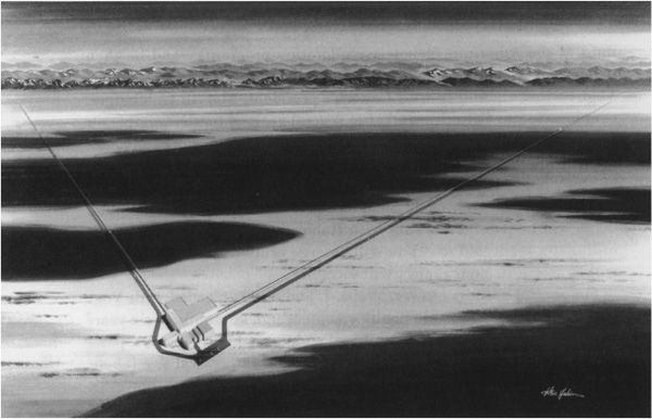
10.8 Artist’s conception of LIGO’s L-shaped vacuum system and the experimental facilities at the corner of the L, near Hanford, Washington. [Courtesy LIGO Project, California Institute of Technology.]
Although two facilities are sufficient to detect a gravitational wave, at least three and preferably four are required, at widely separated sites, to fully decode the wave’s symphony, that is, to extract all the information the wave carries. A joint French/Italian team will build the third facility, named VIRGO, 11 near Pisa, Italy. VIRGO and LIGO together will form an international network for extracting the full information. Teams in Britain, Germany, Japan, and Australia are seeking funds to build additional facilities for the network.
It might seem audacious to construct such an ambitious network for a type of wave that nobody has ever seen. Actually, it is not audacious at all. Gravitational waves have already been proved to exist by astronomical observations for which Joseph Taylor and Russell Hulse of Princeton University won the 1993 Nobel Prize. Taylor and Hulse, using a radio telescope, found two neutron stars, one of them a pulsar, which orbit each other once each 8 hours; and by exquisitely accurate radio measurements, they verified that the stars are spiraling together at precisely the rate (2.7 parts in a billion per year) that Einstein’s laws predict they should, due to being continually kicked by gravitational waves that they emit into the Universe. Nothing else, only tiny gravitational-wave kicks, can explain the stars’ inspiral.
![]()
W hat will gravitational-wave astronomy be like in the early 2000s? The following scenario is plausible:
By 2007, eight interferometers, each several kilometers long, are in full-time operation, scanning the skies for incoming bursts of gravitational waves. Two are operating in the vacuum facility in Pisa, Italy, two in Livingston, Louisiana, in the southeastern United States, two in Hanford, Washington, in the northwestern United States, and two in Japan. Of the two interferometers at each site, one is a “workhorse” instrument that monitors a wave’s oscillations between about 10 cycles per second and 1000; the other, only recently developed and installed, is an advanced, “specialty” interferometer that zeroes in on oscillations between 1000 and 3000 cycles per second.
A train of gravitational waves sweeps into the solar system from a distant, cosmic source. Each wave crest hits the Japanese detectors first, then sweeps through the Earth to the Washington detectors, then Louisiana, and finally Italy. For roughly a minute, crest is followed by trough is followed by crest. The masses in each detector wiggle ever so slightly, perturbing their laser beams and hence perturbing the light that enters the detector’s photodiode. The eight photodiode outputs are transmitted by satellite links to a central computer, which alerts a team of scientists that another minute-long gravitational-wave burst has arrived at Earth, the third one this week. The computer combines the eight detectors’ outputs to produce four things: a best-guess location for the burst’s source on the sky; an error box for that best-guess location; and two waveforms —two oscillating curves, analogous to the oscillating curve that you obtain if you examine the sounds of a symphony on an oscilloscope. The history of the source is encoded in these waveforms (Figure 10.9).
There are two waveforms because a gravitational wave has two polarizations. If the wave travels vertically through an interferometer, one polarization describes tidal forces that oscillate along the east—west and north-south directions; the other describes tidal forces oscillating along the northeast—southwest and northwest—southeast directions. Each detector, with its own orientation, feels some combination of these two polarizations; and from the eight detector outputs, the computer reconstructs the two waveforms.
The computer then compares the waveforms with those in a large catalog, much as a bird watcher identifies a bird by comparing it with pictures in a book. The catalog has been produced by simulations of sources on computers, and by five years of previous experience monitoring gravitational waves from colliding and coalescing black holes, colliding and coalescing neutron stars, spinning neutron stars (pulsars), and supernova explosions. The identification of this burst is easy (some others, for example, from supernovae, are far harder). The waveforms show the unmistakable, unique signature of two black holes coalescing.
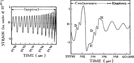
10.9 One of the two waveforms produced by the coalescence of two black holes. The wave is plotted upward in units of 10 −21 time is plotted horizontally in units of seconds. The first graph shows only the last 0.1 second of the inspiral part of the waveform; the preceding minute of the waveform is similar, with gradually Increasing amplitude and frequency. The second graph shows the last 0.01 second, on a stretched-out scale. The Inspiral and Ringdown segments of the waveform are well understood, in 1993, from solutions of the Einstein field equation. The coalescence segment is not at all understood (the curve shown is my own fantasy); future supercomputer simulations will attempt to compute it. In the text these simulations are presumed to have been successful in the early twenty-first century.
The waveforms have three segments:
• The minute-long first segment (of which only the last 0.1 second is shown in Figure 10.9) has oscillating strains that gradually grow in amplitude and frequency; these are precisely the waveforms expected from the inspiral of two objects in a binary orbit. The fact that alternate waves are smaller and larger indicates that the orbit is somewhat elliptical rather than circular.
• The O.Ol-second-long middle segment matches almost perfectly the waveforms predicted by recent (early twenty-first century) supercomputer simulations of the coalescence of two black holes to form one; according to the simulations, the humps marked “H” signal the touching and merging of the holes’ horizons. The double wiggles marked “D,” however, are a new discovery, the first one made by the new specialty interferometers. The older, workhorse interferometers had never been able to detect these wiggles because of their high frequency, and they had never yet been seen in any supercomputer simulations. They are a new challenge for theorists to explain. They might be the first hints of some previously unsuspected quirk in the nonlinear vibrations of the colliding holes’ spacetime curvature. Theorists, intrigued by this prospect, will go back to their simulations and search for signs of such doublet wiggles.
• The 0.03-second-long third segment (of which only the beginning is shown in Figure 10.9) consists of oscillations with fixed frequency and gradually dying amplitude. This is precisely the wave form expected when a deformed black hole pulsates to shake off its deformations, that is, as it rings down like a struck bell. The pulsations consist of two dumbbell-type protrusions that circulate around and around the hole’s equator and gradually die out as ripples of curvature carry away their energy (Figure 10.2 above).
From the details of the waveforms, the computer extracts not only the history of the inspiral, coalescence, and ringdown; it also extracts the masses and spin rates of the initial holes and the final hole. The initial holes each weighed 25 times what the Sun weighs, and were slowly spinning. The final hole weighs 46 times what the Sun weighs and is spinning at 78 percent of the maximum allowed rate. Four solar masses’ worth of energy (2 × 25 - 46 = 4) were converted into ripples of curvature and carried away by the waves. The total surface area of the initial holes was 136,000 square kilometers. The total surface area of the final hole is larger, as demanded by the second law of black-hole mechanics (Chapter 12 ): 144,000 square kilometers. The waveforms also reveal the distance of the hole from Earth: 1 billion light-years, a result accurate to about 20 percent. The waveforms tell us that we on Earth were looking down nearly perpendicularly onto the plane of the orbit, and are now looking down the north pole of the spinning hole; and they show that the holes’ orbit had an eccentricity (elongation) of 30 percent.
The computer determines the holes’ location on the sky from the wave crests’ times of arrival in Japan, Washington, Louisiana, and Italy. Since Japan was hit first, the holes were more or less overhead in Japan, and underfoot in America and Europe. A detailed analysis of the arrival times gives a best-guess location for the source, and an error box around that location of 1 degree in size. Had the holes been smaller, their waveforms would have oscillated more rapidly and the error box would have been tighter, but for these big holes 1 degree is the best the network can do. In another ten years, when an interferometric detector is operating on the Moon, the error boxes will be reduced in size along one side by a factor of 100.
Because the holes’ orbit was elongated, the computer concludes that the two holes were captured into orbit around each other only a few hours before they coalesced and emitted the burst. (If they had been orbiting each other for longer than a few hours, the push of gravitational waves departing from the binary would have made their orbit circular.) Recent capture means the holes were probably in a dense cluster of black holes and massive stars at the center of some galaxy.
The computer therefore examines catalogs of optical galaxies, radio galaxies, and X-ray galaxies, searching for any that reside in the 1 -degree error box, are between 0.8 and 1.2 billion light-years from Earth, and have peculiar cores. Forty candidates are found and turned over to astronomers. For the next few years these forty candidates will be studied in detail, with radio, millimeter, infrared, optical, ultraviolet, X-ray, and gamma-ray telescopes. Gradually it will become clear that one of the candidate galaxies has a core in which a massive agglomerate of gas and stars was beginning, when the light we now see left the galaxy, a million-year-Iong phase of violent evolution—an evolution that will trigger the birth of a gigantic black hole, and then a quasar. Thanks to the burst of gravitational waves which identified this specific galaxy as interesting, astronomers can now begin to unravel the details of how gigantic black holes are born.
1.
The factor
![]() comes from detailed calculations with the Einstein field equation. It includes a factor 1/(2π), which is approximately
comes from detailed calculations with the Einstein field equation. It includes a factor 1/(2π), which is approximately
![]() to convert the hole’s circumference into a radius, and an additional factor
to convert the hole’s circumference into a radius, and an additional factor
![]() that arises from details of the Einstein field equation.
that arises from details of the Einstein field equation.
2. Their lasers actually produced microwaves (short-wavelength radio waves) rather than light, and thus were called masers rather than “lasers.” “Real” lasers, the kind that produce light, were not successfully constructed until several years later.
3. Braginsky has a remarkable mastery of the nuances of the English language; he can construct an eloquent English phrase to describe a new idea far more readily than most Americans or Britons.
4. A key foundation for our idea came from a colleague, William Unruh, at the University of British Columbia. The development of the idea and its consequences was carried out jointly by Caves, me, and three others who were gathered around the lunch table with us when we discovered it: Ronald Drever, Vernon Sandberg, and Mark Zimmermann.
5. The full idea is described by Caves et al. (1980) and by Braginsky, Vorontsov, and Thorne (1980).
6. These differences, their consequences, and the details of the waves to be expected from various astrophysical sources have been elucidated by a number of theorists including, among others, Thibault Damour in Paris, Leonid Grishchuk in Moscow, Takashi Nakamura in Kyoto, Bernard Schutz in Wales, Stuart Shapiro in Ithaca, New York, Clifford Will in St. Louis, and me.
7. Below about one cycle per second, the wires that suspend the masses prevent them from wiggling in response to the waves.
8. Actually, the details of the improvement are far more complicated than this, and the resulting sensitivity enhancement is far more difficult to achieve than these words suggest; however, this description is roughly correct.
9. Though with a close link, through Drever, between the Glasgow and Caltech teams.
10. These, as of 1993, include Braginsky’s group in Moscow, a group led by Bob Byers at Stanford University, a group led by Jim Faller at the University of Colorado, a group led by Peter Saulson at Syracuse University, and a group led by Sam Finn at Northwestern University.
11. It is named for the Virgo cluster of galaxies, from which waves might be detected.
11
![]()
in which spacetime is viewed as
curved on Sundays and flat on Mondays,
and horizons are made from
vacuum on Sundays and charge on Mondays,
but Sunday’s experiments and Monday’s experiments
agree in all details
I s spacetime really curved? Isn’t it conceivable that spacetime is actually flat, but the clocks and rulers with which we measure it, and which we regard as peifect in the sense of Box 11.1, are actually rubbery? Might not even the most perfect of clocks slow down or speed up, and the most perfect of rulers shrink or expand, as we move them from point to point and change their orientations? Wouldn’t such distortions of our clocks and rulers make a truly flat spacetime appear to be curved?
Yes.
Figure 11.1 gives a concrete example: the measurement of circumferences and radii around a nonspinning black hole. On the left is shown an embedding diagram for the hole’s curved space. The space is curved in this diagram because we have chosen to define distances as though our rulers were not rubbery, as though they always hold their lengths fixed no matter where we place them and how we orient them. The rulers show the hole’s horizon to have a circumference of 100 kilometers A circle of twice this circumference, 200 kilometers, is drawn around the hole, and the radial distance from the horizon to that circle is measured with a perfect ruler; the result is 37 kilometers. If space were flat, that radial distance would have to be the radius of the outside circle, 200/π kilometers, minus the radius of the horizon, 100/π kilometers; that is, it would have to be 200/π – 100/π = 16 kilometers (approximately). To accommodate the radial distance’s far larger, 37-kilometer size, the surface must have the curved, trumpet-horn shape shown in the diagram
Box 11.1
Perfection of Rulers and Clocks
By “perfect clocks” and “perfect rulers” I shall mean, in this book, clocks and rulers that are perfect in the sense that the world’s best clock makers and ruler makers understand: Perfection is to be judged by comparison with the behaviors of atoms and molecules.
More specifically, perfect clocks must tick at a uniform rate when compared with the oscillations of atoms and molecules. The world’s best atomic clocks are designed to do just that. Since the oscillations of atoms and molecules are controlled by what I called in earlier chapters the “rate of flow of time,” this means that perfect clocks measure the “time” part of Einstein’s curved spacetime.
The markings on perfect rulers must have uniform and standard spacings when compared to the wavelengths of the light emitted by atoms and molecules, for example, uniform spacings relative to the “21-centimeter-wavelength” light emitted by hydrogen molecules. This is equivalent to requiring that when one holds a ruler at some fixed, standard temperature (say, zero degrees Celsius), it contain always the same fixed number of atoms along its length between markings; and this, in turn, guarantees that perfect rulers measure the spatial lengths of Einstein’s curved space-time.
The body of this chapter introduces the concept of “true” times and “true” lengths. These are not necessarily the times and lengths measured by perfect clocks and perfect rulers, that is, not necessarily the times and lengths based on atomic and molecular standards, that is, not necessarily the times and lengths embodied in Einstein’s curved spacetime.
If space is actually flat around the black hole, but our perfect rulers are rubbery and thereby fool us into thinking space is curved, then the true geometry of space must be as shown on the right in Figure 11.1, and the true distance between the horizon and the circle must be 16 kilometers, as demanded by the flat-geometry laws of Euclid. However, general relativity insists that our perfect rulers not measure this true distance. Take a ruler and lay it down circumferentially around the hole just outside the horizon (curved thick black strip with ruler markings in right part of Figure 11.1). When oriented circumferentially like this, it does measure correctly the true distance. Cut the ruler off at 37 kilometers length, as shown. It now encompasses 37 percent of the distance around the hole. Then turn the ruler so it is oriented radially (straight thick black strip with ruler markings in Figure 11.1). As it is turned, general relativity requires that it shrink. When pointed radially, its true length must have shrunk to 16 kilometers, so it will reach precisely from the horizon to the outer circle. However, the scale on its shrunken surface must claim that its length is still 37 kilometers, and therefore that the distance between horizon and circle is 37 kilometers. People like Einstein who are unaware of the ruler’s rubbery nature, and thus believe its inaccurate measurement, conclude that space is curved. However, people like you and me, who understand the rubberiness, know that the ruler has shrunk and that space is really flat.
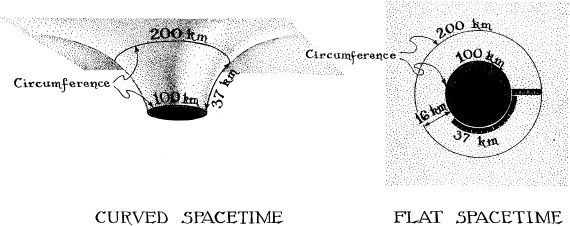
11.1 Length measurements in the vicinity of a black hole from two different viewpoints. Left: Spacetime is regarded as truly curved, and perfect rulers measure precisely the lengths of the true spacetime. Right: Spacetime is regarded as truly flat and perfect rulers are rubbery. A 57-km-Iong perfect ruler, when oriented in a circumferential direction, measures precisely the lengths of the true, flat spacetime. However, when oriented radially, it shrinks by an amount that is greater the nearer it is to the hole, and therefore it reports radial lengths that are larger than the true ones (it reports 37 km rather than the true 16 km in the case shown).
What could possibly make the ruler shrink, when its orientation changes? Gravity, of course. In the flat space of the right half of Figure 11.1 there resides a gravitational field that controls the sizes of fundamental particles, atomic nuclei, atoms, molecules, everything, and forces them all to shrink when laid out radially. The amount of shrinkage is great near a black hole, and smaller farther away, because the shrinkage-controlling gravitational field is generated by the hole, and its influence. declines with distance.
The shrinkage-controlling gravitational field has other effects. When a photon or any other particle flies past the hole, this field pulls on it and deflects its trajectory. The trajectory is bent around the hole; it is curved, as measured in the hole’s true, flat spacetime geometry. However, people like Einstein, who take seriously the measurements of their rubbery rulers and clocks, regard the photon as moving along a straight line through curved spacetime.
What is the real, genuine truth? Is spacetime really flat, as the above paragraphs suggest, or is it really curved? To a physicist like me this is an uninteresting question because it has no physical consequences. Both viewpoints, curved spacetime and flat, give precisely the same predictions for any measurements performed with perfect rulers and clocks, and also (it turns out) the same predictions for any measurements performed with any kind of physical apparatus whatsoever. For example, both viewpoints agree that the radial distance between the horizon and the circle in Figure 11.1, as measured by a perfect ruler, is 37 kilometers. They disagree as to whether that measured distance is the “real” distance, but such a disagreement is a matter of philosophy, not physics. Since the two viewpoints agree on the results of all experiments, they are physically equivalent. Which viewpoint tells the “real truth” is irrelevant for experiments; it is a matter for philosophers to debate, not physicists. Moreover, physicists can and do use the two viewpoints interchangeably when trying to deduce the predictions of general relativity.
T he mental processes by which a theoretical physicist works are beautifully described by Thomas Kuhn’s concept of a paradigm Kuhn, who received his Ph.D. in physics from Harvard in 1949 and then became an eminent historian and philosopher of science, introduced the concept of a paradigm in his 1962 book The Structure of Scientific Revolutions —one of the most insightful books I have ever read.
A paradigm is a complete set of tools that a community of scientists uses in its research on some topic, and in communicating the results of its research to others. The curved spacetime viewpoint on general relativity is one paradigm; the flat spacetime viewpoint is another. Each of these paradigms includes three basic elements: a set of mathematically formulated laws of physics; a set of pictures (mental pictures, verbal pictures, drawings on paper) which give us insight into the laws and help us communicate with each other; and a set of exemplars —past calculations and solved problems, either in textbooks or in published scientific articles, which the community of relativity experts agrees were correctly done and were interesting, and which we use as patterns for our future calculations.
The curved spacetime paradigm is based on three sets of mathematically formulated laws: Einstein’s field equation, which describes how matter generates the curvature of spacetime; the laws which tell us that perfect rulers and perfect clocks measure the lengths and the times of Einstein’s curved spacetime; and the laws which tell us how matter and fields move through curved spacetime, for example, that freely moving bodies travel along straight lines (geodesics). The flat spacetime paradigm is also based on three sets of laws: a law describing how matter, in flat spacetime, generates the gravitational field; laws describing how that field controls the shrinkage of perfect rulers and the dilation of the ticking rates of perfect clocks; and laws describing how the gravitational field also controls the motions of particles and fields through flat spacetime.
The pictures in the curved spacetime paradigm include the embedding diagrams drawn in this book (for example, the left half of Figure 11.1) and the verbal descriptions of spacetime curvature around black holes (for example, the “tornado-like swirl of space around a spinning black hole”). The pictures in the flat spacetime paradigm include the right half of Figure 11.1, with the ruler that shrinks when it turns from circumferential orientation to radial, and the verbal description of “a gravitational field controlling the shrinkage of rulers.”
The exemplars of the curved spacetime paradigm include the calculation, found in most relativity textbooks, by which one derives Schwarzschild’s solution to the Einstein field equation, and the calculations by which Israel, Carter, Hawking, and others deduced that a black hole has no “hair.” The flat spacetime exemplars include textbook calculations of how the mass of a black hole or other body changes when gravitational waves are captured by it, and calculations by Clifford Will, Thibault Damour, and others of how neutron stars orbiting each other generate gravitational waves (waves of shrinkage-producing field).
Each piece of a paradigm—its laws, its pictures, and its exemplars—is crucial to my own mental processes when I’m doing research. The pictures (mental and verbal as well as on paper) act as a general compass. They give me intuition as to how the Universe probably behaves; I manipulate them, along with mathematical doodlings, in search of interesting new insights. If I find, from the pictures and doodlings, an insight worth pursuing (for example, the hoop conjecture in Chapter 7 ), I then try to verify or refute it by careful mathematical calculations based on the paradigm’s mathematically formulated laws of physics. I pattern my careful calculations after the paradigm’s exemplars. They tell me what level of calculational precision is likely to be needed for reliable results. (If the precision is too poor, the results may be wrong; if the precision is too high, the calculations may eat up valuable time unnecessarily.) The exemplars also tell me what kinds of mathematical manipulations are likely to get me through the morass of mathematical symbols to my goal. Pictures also guide the calculations; they help me find shortcuts and avoid blind alleys. If the calculations verify or at least make plausible my new insight, I then communicate the insight to relativity experts by a mixture of pictures and calculations, and I communicate to others, such as readers of this book, solely with pictures—verbal pictures and drawings.
The flat spacetime paradigm’s laws of physics can be derived, mathematically, from the curved spacetime paradigm’s laws, and conversely. This means that the two sets of laws are different mathematical representations
of the same physical phenomena, in somewhat the same sense as 0.001 and ![]() are different mathematical representations of the same number. However, the mathematical formulas for the laws look very different in the two representations, and the pictures and exemplars that accompany the two sets of laws look very different.
are different mathematical representations of the same number. However, the mathematical formulas for the laws look very different in the two representations, and the pictures and exemplars that accompany the two sets of laws look very different.
As an example, in the curved spacetime paradigm, the verbal picture of Einstein’s field equation is the statement that “mass generates the curvature of spacetime.” When translated into the language of the flat spacetime paradigm, this field equation is described by the verbal picture “mass generates the gravitational field that governs the shrinkage of rulers and the dilation of the ticking of clocks.” Although the two versions of the Einstein field equation are mathematically equivalent, their verbal pictures differ profoundly.
It is extremely useful, in relativity research, to have both paradigms at one’s fingertips. Some problems are solved most easily and quickly using the curved spacetime paradigm; others, using flat spacetime. Black-hole problems (for example, the discovery that a black hole has no hair) are most amenable to curved spacetime techniques; gravitational-wave problems (for example, computing the waves produced when two neutron stars orbit each other) are most amenable to flat spacetime techniques. Theoretical physicists, as they mature, gradually build up insight into which paradigm will be best for which situation, and they learn to flip their minds back and forth from one paradigm to the other, as needed. They may regard spacetime as curved on Sunday, when thinking about black holes, and as flat on Monday, when thinking about gravitational waves. This mind-flip is similar to that which one experiences when looking at a drawing by M. C. Escher, for example, Figure 11.2.
Since the laws that underlie the two paradigms are mathematically equivalent, we can be sure that when the same physical situation is analyzed using both paradigms, the predictions for the results of experiments will be identically the same. We thus are free to use the paradigm that best suits us in any given situation.
This freedom carries power. That is why physicists were not content with Einstein’s curved spacetime paradigm, and have developed the flat spacetime paradigm as a supplement to it.
N ewton’s description of gravity is yet another paradigm. It regards space and time as absolute, and gravity as a force that acts instantaneously between two bodies (“action at a distance,” Chapters 1 and 2 ).
The Newtonian paradigm for gravity, of course, is not equivalent to Einstein’s curved spacetime paradigm; the two give different predictions for the outcomes of experiments. Thomas Kuhn uses the phrase scientific revolution to describe the intellectual struggle by which Einstein invented his paradigm and convinced his colleagues that it gives a more nearly correct description of gravity than the Newtonian paradigm (Chapter 2 ). Physicists’ invention of the flat spacetime paradigm was not a scientific revolution in this Kuhnian sense, because the flat spacetime paradigm and the curved spacetime paradigm give precisely the same predictions.
11.2 A drawing by M. C. Escher. One can experience a mind-flip by looking at this drawing, first from one point of view (for example, with the flowing stream at the same height as the waterfall’s top) and then from another (with the stream at the height of the waterfall’s bottom). This mind-flip is somewhat like the one a theoretical physicist experiences when switching from the curved spacetime paradigm to the flat spacetime paradigm. [© 1961 M. C. Escher Foundation–Baarn-Holland. All rights reserved.]
When gravity is weak, the predictions of the Newtonian paradigm and Einstein’s curved spacetime paradigm are almost identical, and correspondingly the two paradigms are very nearly mathematically equivalent. Thus it is that, when studying gravity in the solar system, physicists often switch back and forth with impunity between the Newtonian paradigm, the curved spacetime paradigm, and also the flat spacetime paradigm, using at any time whichever one strikes their fancy or seems the more insightful. 1
S ometimes people new to a field of research are more open-minded than the old hands. Such was the case in the 1970s, when new people had insights that led to a new paradigm for black holes, the membrane paradigm.
In 1971 Richard Hanni, an undergraduate at Princeton University, together with Remo Ruffini, a postdoc, noticed that a black hole’s horizon can behave somewhat like an electrically conducting sphere. To understand this peculiar behavior, recall that a positively charged metal pellet carries an electric field which repels protons but attracts electrons. The pellet’s electric field can be described by field lines, analogous to those of a magnetic field. The electric field lines point in the direction of the force that the field exerts on a proton (and oppositely to the force exerted on an electron), and the density of field lines is proportional to the strength of the force. If the pellet is alone in flat spacetime, its electric field lines point radially outward (Figure 11.3a). Correspondingly, the electric force on a proton points radially away from the pellet, and since the density of field lines decreases inversely with the square of the distance from the pellet, the electric force on a proton also decreases inversely with the square of the distance.
Now bring the pellet close to a metal sphere (Figure 11.3b). The sphere’s metal surface is made of electrons that can move about on the sphere freely, and positively charged ions that cannot. The pellet’s electric field pulls a number of the sphere’s electrons into the pellet’s vicinity, leaving excess ions everywhere else on the sphere; in other words, it polarizes 2 the sphere.
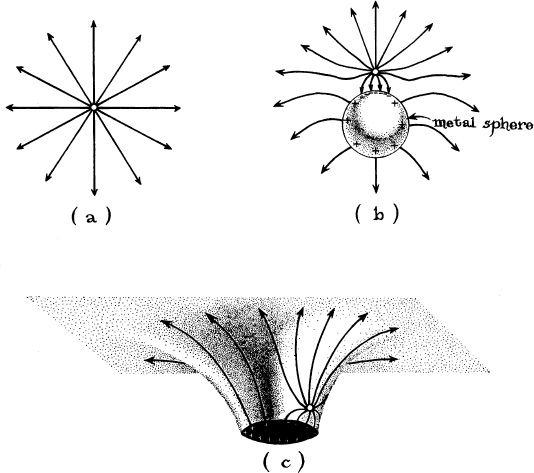
11.3 (a) The electric field lines produced by a positively charged metal pellet at rest, alone, in flat spacetime. (b) The electric field lines when the pellet is at rest just above an electrically conducting, metal sphere in flat spacetime. The pellet’s electric field polarizes the sphere. (c) The electric field lines when the pellet is at rest just above the horizon of a black hole. The pellet’s electric field appears to polarize the horizon.
In 1971 Hanni and Ruffirti, and independently Robert Wald of Princeton University and Jeff Cohen of the Princeton Institute for Advanced Study, computed the shapes of the electric field lines produced by a charged pellet near the horizon of a nonspinning black hole. Their computations, based on the standard curved spacetime paradigm, revealed that the curvature of spacetime distorts the field lines in the manner shown in Figure 11.3c. Hanni and Ruffini, noticing the similarity to the field lines in Figure 11.3b [look at diagram (c) from below, and it will be nearly the same as diagram (b)], suggested that we can think of a black hole’s horizon in the same manner as we think of a metal sphere; that is, we can regard the horizon as a thin membrane composed of positively and negatively charged particles, a membrane similar to the sphere’s metal. Normally there are equal numbers of positive and negative particles everywhere on the membrane, that is, there is no net charge on any region of the membrane. However, when the pellet is brought near the horizon, excess negative particles move into the region below the pellet, leaving excess positive particles everywhere else on the membrane; the horizon’s membrane thereby gets polarized; and the total set of field lines produced by the pellet’s charges and the horizon’s charges takes the form of diagram (c).
When I, as an old hand at relativity theory, heard this story, I thought it ludicrous. General relativity insists that, if one falls into a black hole, one will encounter nothing at the horizon except spacetime curvature. One will see no membrane and no charged particles. Thus, the Hanni–Ruffini description of why the pellet’s electric field lines are bent can have no basis in reality. It is pure fiction. The cause of the field lines’ bending, I was sure, is spacetime curvature and nothing else: The field lines bend down toward the horizon in diagram (c) solely because tidal gravity pulls on them, and not because they are being attracted to some polarized charge in the horizon. The horizon cannot possess any such polarized charge; I was sure of it. I was wrong.
Five years later Roger Blandford and a graduate student, Roman Znajek, at Cambridge University discovered that magnetic fields can extract the spin energy of a black hole and use it to power jets (the Blandford-Znajek process, Chapter 9 and Figure 11.4a). Blandford and Znajek also found by curved spacetime calculations that, as the energy is extracted, electric currents flow into the horizon near the hole’s poles (in the form of positively charged particles falling inward), and currents flow out of the horizon near the equator (in the form of negatively charged particles falling inward). It was as though the black hole were part of an electric circuit.
The calculations showed, moreover, that the hole behaved as though it were a voltage generator in the circuit (Figure 11.4b). This black-hole voltage generator drove current out of the horizon’s equator, then up magnetic field lines to a large distance from the hole, then through plasma (hot, electrically conducting gas) to other field lines near the hole’s spin axis, then down those field lines and into the horizon. The magnetic field lines were the wires of the electric circuit, the plasma was the load that extracts power from the circuit, and the spinning hole was the power source.
From this viewpoint (Figure 11.4b), it is the power carried by the circuit that accelerates the plasma to form jets. From the viewpoint of Chapter 9 (Figure 11.4a), it is the spinning magnetic field lines, whipping around and around, that accelerate the plasma. The two viewpoints are just different ways of looking at the same thing. The power comes ultimately from the hole’s spin in both cases. Whether one thinks of the power as carried by the circuit or as carried by the spinning field lines is a matter of taste.
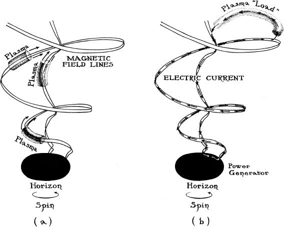
11.4 Two viewpoints on the Blandford–Znajek process by which a spinning, magnetized black hole can produce jets. (a) The hole’s spin creates a swirl of space which forces magnetic fields threading the hole to spin. The spinning fields’ centrifugal forces then accelerate plasma to high speeds (compare with Figure 9.7d). (b) The magnetic fields and the swirl of space together generate a large voltage difference between the hole’s poles and equator; in effect, the hole becomes a voltage and power generator. This voltage drives current to flow in a circuit. The circuit carries electrical power from the black hole to the plasma, and that power accelerates the plasma to high speeds.
The electric circuit description, although based on the standard curved spacetime laws of physics, was totally unexpected, and the flow of current through the black hole—inward near the poles and outward near the equator—seemed very peculiar. During 1977 and 1978, Znajek and, independently, Thibault Damour (a recent PhD at the Obser-vatoire de Paris in France) puzzled over this peculiarity. While trying to understand it, they independently translated the curved spacetime equations, which describe the spinning hole and its plasma and magnetic field, into an unfamiliar form with an intriguing pictorial interpretation: The current, when it reaches the horizon, does not enter the hole. Instead, it attaches itself to the horizon, where it is carried by the kinds of horizon charges previously imagined by Hanni and Ruffini. This horizon current flows from the pole to the equator, where it exits up the magnetic field lines. Moreover, Damour and Znajek discovered, the laws that govern the horizon’s charge and current are elegant versions of the flat spacetime laws of electricity and magnetism: They are Gauss’s law, Ampère’s law, Ohm’s law, and the law of charge conservation (Figure 11.5).
Damour and Znajek did not assert that a being who falls into the black hole will encounter a membrane-like horizon with electric charges and currents. Rather, they asserted that if one wishes to figure out how electricity, magnetism, and plasmas behave outside a black hole, it is useful to regard the horizon as a membrane with charges and currents.
When I read the technical articles by Damour and Znajek, I suddenly understood: They, and Hanni and Ruffini before them, were discovering the foundations of a new paradigm for black holes. The paradigm was fascinating. It captivated me. Unable to resist its allure, I spent much of the 1980s, together with Richard Price, Douglas Mac-donald, Ian Redmount, Wai-Mo Suen, Ronald Crowley, and others, bringing it into a polished form and writing a book on it, Black Holes: The Membrane Paradigm
The laws of black-hole physics, written in this membrane paradigm, are completely equivalent to the corresponding laws of the curved spacetime paradigm—so long as one restricts attention to the hole’s exterior. Consequently, the two paradigms give precisely the same predictions for the outcomes of all experiments or observations that anyone might make outside a black hole—including all astronomical observations made from Earth. When thinking about astronomy and astrophysics, I find it useful to keep both paradigms at hand, membrane and curved spacetime, and to do Escher-type mind-flips back and forth between them. The curved spacetime paradigm, with its horizons made from curved empty spacetime, may be useful on Sunday, when I am puzzling over the pulsations of black holes. The membrane paradigm, with horizons made from electrically charged membranes, may be useful on Monday, when I am puzzling over a black hole’s production of jets. And since the predictions of the two paradigms are guaranteed to be the same, I can use each day whichever one best suits my needs.
11.5 The laws governing electric charge and current on a black hole’s membrane-like horizon: (a) Gauss’s law—the horizon has precisely the right amount of surface charge to terminate all electric field lines which intersect the horizon, so they do not extend into the hole’s interior; compare with Figure 11.3. (b) Ampere’s law—the horizon has precisely the right amount of surface current to terminate that portion of the magnetic field which is parallel to the horizon, so there is no parallel field below the horizon. (c) Ohm’s law—the surface current is proportional to the part of the electric field which is tangential to the surface; the proportionality constant is a resistivity of 377 ohms. (d) Charge conservation—no charge is ever lost or created; all positive charge that enters the horizon from the outside Universe becomes attached to the horizon, and moves around on it, until it exits back into the outside Universe (in the form of negative charge falling inward to neutralize the positive charge).
Not so inside a black hole. Any being who falls into a hole will discover that the horizon is not a charge-endowed membrane, and that inside the hole the membrane paradigm completely loses its power. However, infalling beings pay a price to discover this: They cannot publish their discovery in the scientific journals of the outside Universe
1. pare with the last section of Chapter 1 , “The Nature of Physical Law.”
2. This is a different usage of the word “polarize” from that of “polarized gravitational waves” and “polarized light” ( Chapter 10 ).
12
![]()
in which a black-hole horizon
is clothed in an atmosphere
of radiation and hot particles
that slowly evaporate,
and the hole shrinks
and then explodes
Black Holes Grow
T he Idea hit Stephen Hawking one evening in November 1970, as he was preparing for bed. It hit with such force that he was left almost gasping for air. Never before or since has an idea come to him so quickly.
Preparing for bed was not easy. Hawking’s body is afflicted with amyotrophic lateral sclerosis (ALS), a disease that gradually destroys the nerves which control the body’s muscles and leaves the muscles, one after another, to waste away in disuse. He moved slowly, with legs wobbling and at least one hand always firmly grasping a countertop or bedpost, as he brushed his teeth, disrobed, struggled into his pajamas, and climbed into bed. That evening he moved even more slowly than usual, since his mind was preoccupied with the Idea. The Idea excited him. He was ecstatic, but he didn’t tell his wife, Jane; that would have made him most unpopular, since he was supposed to be concentrating on getting to bed.
He lay awake for many hours that night. He couldn’t sleep. His mind kept roaming over the Idea’s ramifications, its connections to other things.
The Idea had been triggered by a simple question. How much gravitational radiation (ripples of spacetime curvature) can two black holes produce, when they collide and coalesce to form a single hole? Hawking had been vaguely aware for some time that the single final hole would have to be larger, in some sense, than the “sum” of the two original holes, but in what sense, and what could that tell him about the amount of gravitational radiation produced?
Then, as he was preparing for bed, it had hit him. Suddenly, a series of mental pictures and diagrams had coalesced in his mind to produce the Idea: It was the area of the hole’s horizon that would be larger. He was sure of it; the pictures and diagrams had coalesced into an unequivocal, mathematical proof. No matter what the masses of the two original holes might be (the same or very different), and no matter how the holes might spin (in the same direction or opposite or not at all), and no matter how the holes might collide (head-on or at a glancing angle), the area of the final hole’s horizon must always be larger than the sum of the areas of the original holes’ horizons. So what? So a lot, Hawking realized as his mind roamed over the ramifications of this area-increase theorem
First of all, in order for the final hole’s horizon to have a large area, the final hole must have a large mass (or equivalently a large energy), which means that not too much energy could have been ejected, as gravitational radiation. But “not too much” was still quite a bit. By combining his new area-increase theorem with an equation that describes the mass of a black hole in terms of its surface area and spin, Hawking deduced that as much as 50 percent of the mass of the two original holes could be converted to gravitational-wave energy, leaving as little as 50 percent behind in the mass of the final hole. 1
There were other ramifications Hawking realized in the months that followed his sleepless November night. Most important, perhaps, was a new answer to the question of how to define the concept of a hole’s horizon when the hole is “dynamical,” that is, when it is vibrating wildly (as it must during collisions), or when it is growing rapidly (as it will when it is first being created by an imploding star).
Precise and fruitful definitions are essential to physics research. Only after Hermann Minkowski had defined the absolute interval between two events (Box 2.1) could he deduce that, although space and time are “relative,” they are unified into an “absolute” spacetime. Only after Einstein had defined the trajectories of freely falling particles to be straight lines (Figure 2.2) could he deduce that spacetime is curved (Figure 2.5), and thereby develop his laws of general relativity. And only after Hawking had defined the concept of a dynamical hole’s horizon could he and others explore in detail how black holes change when pummeled by collisions or by infalling debris.
Before November 1970, most physicists, following Roger Penrose’s lead, had thought of a hole’s horizon as “the outermost location where photons trying to escape the hole get pulled inward by gravity.” This old definition of the horizon was an intellectual blind alley, Hawking realized in the ensuing months, and to brand it as such he gave it a new, slightly contemptuous name, a name that would stick. He called it the apparent horizon. 2
Hawking’s contempt had several roots. First, the apparent horizon is a relative concept, not an absolute one. Its location depends on the observers’ reference frame; observers falling into the hole might see it at a different location from observers at rest outside the hole. Second, when matter falls into the hole, the apparent horizon can jump suddenly, without warning, from one location to another—a rather bizarre behavior, one not conducive to easy insights. Third and most important, the apparent horizon had no connection at all to the flash of congealing mental pictures and diagrams that had produced Hawking’s New Idea.
Hawking’s new definition of the horizon, by contrast, was absolute (the same in all reference frames), not relative, so he called it the absolute horizon. This absolute horizon is beautiful, Hawking thought. It has a beautiful definition: It is “the boundary in spacetime between events (outside the horizon) that can send signals to the distant Universe and those (inside the horizon) that cannot.” And it has a beautiful evolution: When a hole eats matter or collides with another hole or does anything at all, its absolute horizon changes shape and size in a smooth, continuous way, instead of a sudden, jumping way (Box 12.1). Most important, the absolute horizon meshed perfectly with Hawking’s New Idea:
Box 12.1
Absolute and Apparent Horizons for a Newborn Black Hole
The spacetime diagrams shown below describe the implosion of a spherical star to form a spherical black hole; compare with Figure 6.7. The dotted curves are outgoing light rays; in other words, they are the world lines (trajectories through spacetime) of photons—the fastest signals that can be sent radially outward, toward the distant Universe. For optimal escape, the photons are idealized as not being absorbed or scattered at all by the star’s matter.
The apparent horizon (left diagram) is the outermost location where outgoing light rays, trying to escape the hole, get pulled inward toward the singularity (for example, the outgoing rays QQ′ and RR′). The apparent horizon is created suddenly, full-sized, at E, where the star’s surface shrinks through the critical circumference. The absolute horizon (right diagram) is the boundary between events that can send signals to the distant Universe (for example, events P and S which send signals along the light rays pp′ and SS′) and events that cannot send signals to the distant Universe (for example, Q and R). The absolute horizon is created at the star’s center, at the event labeled C, well before the star’s surface shrinks through the critical circumference. The absolute horizon is just a point when created, but it then expands smoothly, like a balloon being blown up, and emerges through the star’s surface precisely when the surface shrinks through the critical circumference (the circle labeled E). It then stops expanding, and thereafter coincides with the suddenly created apparent horizon.
Hawking could see, in his congealed mental pictures and diagrams, that the areas of absolute horizons (but not necessarily apparent horizons) will increase not only when black holes collide and coalesce, but also when they are being born, when matter or gravitational waves fall into them, when the gravity of other objects in the Universe raises tides on them, and when rotational energy is being extracted from the swirl of space just outside their horizons. Indeed, the areas of absolute horizons will almost always increase, and can never decrease. The physical reason is simple: Everything that a hole encounters sends energy inward through its absolute horizon, and there is no way that any energy can come back out. Since all forms of energy produce gravity, this means that the hole’s gravity is continually being strengthened, and correspondingly, its surface area is continually growing.
Hawking’s conclusion, stated more precisely, was this: In any region of space, and at any moment of time (as measured in anyone’s reference frame), measure the areas of all the absolute horizons of all black holes and add the areas together to get a total area. Then wait however long you might wish, and again measure the areas of all the absolute horizons and add them If no black holes have moved out through the “walls” of your region of space between the measurements, then the total horizon area cannot have decreased, and it almost always will have increased, at least a little bit
Hawking was well aware that the choice of definition of horizon, absolute or apparent, could not influence in any way any predictions for the outcomes of experiments that humans or other beings might perform; for example, it could not influence predictions of the waveforms of gravitational radiation produced in black-hole collisions (Chapter 10 ), nor could it influence predictions of the number of X-rays emitted by hot gas falling into and through a black hole’s horizon (Chapter 8 ). However, the choice of definition could strongly influence the ease with which theoretical physicists deduce, from Einstein’s general relativistic equations, the properties and behaviors of black holes. The chosen definition would become a central tool in the paradigm by which theorists guide their research; it would influence their mental pictures, their diagrams, the words they say when communicating with each other, and their intuitive leaps of insight. And for this purpose, Hawking believed, the new, absolute horizon, with its smoothly increasing area, would be superior to the old, apparent horizon, with its discontinuous jumps in size.
S tephen Hawking was not the first physicist to think about absolute horizons and discover their area increase. Roger Penrose at Oxford had already done so, before Hawking’s sleepless November night. In fact, Hawking’s insights were based largely on foundations laid by Penrose (Chapter 13 ) and a recent conversation with him. However, Penrose had not recognized the power of the area-increase theorem, and so had not perfected nor published it. Why had he missed its power? Because he had not developed any clear mental picture of the absolute horizon’s location. He had missed what Hawking saw so clearly that sleepless night: After black holes collide, their merged absolute horizon should soon settle down into a quiescent location whose surface area can be computed from the standard equations for quiescent black holes.
Werner Israel at the University of Alberta, Canada, also caught a glimpse of the area increase theorem before Hawking; but, failing to recognize its importance, he, too, let it slip by unpublished. Moreover, by contrast with Hawking and Penrose, Israel was still using—indeed, was hypnotized by—the old concept of the apparent horizon, as were all the rest of us relativity theorists. The apparent horizon had played a central role in Penrose’s amazing 1964 discovery that Einstein’s laws force every black hole to have a singularity at its center (Chapter 13 ). The apparent horizon thereby had proved its power. Blinded by that power, we relativists could not conceive of replacing the apparent horizon, as the definition of a black hole’s surface, by the absolute horizon.
We also were paying little attention to the absolute horizon because it violates our cherished notion that an effect should not precede its cause. When matter falls into a black hole, the absolute horizon starts to grow (“effect”) before the matter reaches it (“cause”). The horizon grows in anticipation that the matter will soon be swallowed and will increase the hole’s gravitational pull (Box 12.2). This seeming paradox has a simple origin. The very definition of the absolute horizon depends on what will happen in the future: on whether or not signals will ultimately escape to the distant Universe. In the terminology of philosophers, it is a teleological definition (a definition that relies on “final causes”), and it forces the horizon’s evolution to be teleological. Since teleological viewpoints have rarely if ever been useful in modern physics, the absolute horizon seemed hardly worth exploring.
Box 12.2
Evolution of an Accreting Hole’s Apparent and Absolute Horizons
The spacetime diagram below illustrates the jerky evolution of the apparent horizon and the teleological evolution of the absolute horizon. At some initial moment of time (on a horizontal slice near the bottom of the diagram), an old, nonspinning black hole is surrounded by a thin, spherical shell of matter. The shell is like the rubber of a balloon, and the hole is like a pit at the balloon’s center. The hole’s gravity pulls on the shell (the balloon’s rubber), forcing it to shrink and ultimately be swallowed by the hole (the pit). The apparent horizon (the outermost location at which outgoing light rays—shown dotted—are being pulled inward) jumps outward suddenly, and discontinuously, at the moment when the shrinking shell reaches the location of the final hole’s critical circumference. The absolute horizon (the boundary between events that can and cannot send outgoing light rays to the distant Universe) starts to expand before the hole swallows the shell. It expands in anticipation of swallowing, and then, just as the hole swallows, it comes to rest at the same location as the jumping apparent horizon.
Hawking is a bold thinker. He is far more willing than most physicists to take off in radical new directions, if those directions “smell” right. The absolute horizon smelled right to him, so despite its radical nature, he embraced it, and his embrace paid off. Within a few months, Hawking and James Hartle were able to derive, from Einstein’s general relativity laws, a set of elegant equations that describe how the absolute horizon continuously and smoothly expands and changes its shape, in anticipation of swallowing infalling debris or gravitational waves, or in anticipation of being pulled on by the gravity of other bodies.
I n November 1970, Stephen Hawking was just beginning to reach full stride as a physicist. He had made several important discoveries already, but he was not yet a dominant figure. As we move on through this chapter, we shall watch him become dominant.
How, with his severe disability, has Hawking been able to out-think and out-intuit his leading colleague-competitors, people like Roger Penrose, Werner Israel, and (as we shall see) Yakov Borisovich Zel’-dovich? They had the use of their hands; they could draw pictures and perform many-page-Iong calculations on paper—calculations in which one records many complex intermediate results along the way, and then goes back, picks them up one by one, and combines them to get a final result; calculations that I cannot conceive of anyone doing in his head. By the early 1970s, Hawking’s hands were largely paralyzed; he could neither draw pictures nor write down equations. His research had to be done entirely in his head.
Because the loss of control over his hands was so gradual, Hawking has had plenty of time to adapt. He has gradually trained his mind to think in a manner different from the minds of other physicists: He thinks in new types of intuitive mental pictures and mental equations that, for him, have replaced paper-and-pen drawings and written equations. Hawking’s mental pictures and mental equations have turned out to be more powerful, for some kinds of problems, than the old paper-and-pen ones, and less powerful for others, and he has gradually learned to concentrate on problems for which his new methods give greater power, a power that nobody else can begin to match.
Hawking’s disability has helped him in other ways. As he himself has often commented, it has freed him from the responsibility of lecturing to university students, and he thus has had far more free time for research than his more healthy colleagues. More important, perhaps, his disease in some ways has improved his attitude toward life.
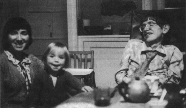
Stephen Hawking with his wife Jane and their son Timothy in Cambridge, England, in 1980. [Photo by Kip Thorne.]
Hawking contracted ALS in 1963, soon after he began graduate school at Cambridge University. ALS is a catch-all name for a variety of motor neuron diseases, most of which kill fairly quickly. Thinking he had only a few years to live, Hawking at first lost his enthusiasm for life and physics. However, by the winter of 1964–65, it became apparent that his was a rare variant of ALS, a variant that saps the central nervous system’s control of muscles over many years’ time, not just a few. Suddenly life seemed wonderful. He returned to physics with greater vigor and enthusiasm than he had ever had as a healthy, devil-may-care undergraduate student; and with his new lease on life, he married Jane Wilde, whom he had met shortly after contracting ALS and with whom he had fallen in love during the early phases of his disease.
Stephen’s marriage to Jane was essential to his success and happiness in the 1960s and 1970s and into the 1980s. She made for them a normal home and a normal life in the midst of physical adversity.
The happiest smile I ever saw in my life was Stephen’s the evening in August 1972 in the French Alps when Jane, I, and the Hawkings’ two oldest children, Robert and Lucy, returned from a day’s excursion into the mountains. Through foolishness we had missed the last ski lift down the mountain, and had been forced to descend about 1000 meters on foot. Stephen, who had fretted about our tardiness, broke out into an enormous smile, and tears came to his eyes, as he saw Jane, Robert, and Lucy enter the dining room where he was poking at his evening meal, unable to eat.
Hawking lost the use of his limbs and then his voice very gradually. In June 1965, when we first met, he walked with a cane and his voice was only slightly shaky. By 1970 he required a four-legged walker. By 1972 he was confined to a motorized wheelchair and had largely lost the ability to write, but he could still feed himself with some ease, and most native English speakers could still understand his speech, though with difficulty. By 1975 he could no longer feed himself, and only people accustomed to his speech could understand it. By 1981 even I was having severe difficulty understanding him unless we were in an absolutely quiet room; only people who were with him a lot could understand with ease. By 1985 his lungs would not remain clear of fluid of their own accord, and he had to have a tracheostomy so they could be cleared regularly by suctioning. The price was high: He completely lost his voice. To compensate, he acquired a computer-driven voice synthesizer with an American accent for which he would apologize sheepishly. He controls the computer by a simple switch clutched in one hand, which he squeezes as a menu of words scrolls by on the computer screen. Grabbing one word after another from the scrolling menu with his switch, he builds up his sentences. It is painfully slow, but effective; he can produce no more than one short sentence per minute, but his sentences are enunciated clearly by the synthesizer, and are often pearls.
As his speech deteriorated, Hawking learned to make every sentence count. He found ways to express his ideas that were clearer and more succinct than the ways he had used in the early years of his disease. With clarity and succinctness of expression came improved clarity of thought, and greater impact on his colleagues—but also a tendency to seem oracular: When he issues a pronouncement on some deep question, we, his colleagues, sometimes cannot be sure, until after much thought and calculation of our own, whether he is just speculating or has strong evidence. He sometimes doesn’t tell us, and we occasionally wonder whether he, with his absolutely unique insights, is playing games with us. He does, after all, still retain a streak of the impishness that made him popular in his undergraduate days at Oxford, and a sense of humor that rarely deserts him, even in times of trial. (Before his tracheostomy, when I began to have trouble understanding his speech, I sometimes found myself saying over and over again, as many as ten times, “Stephen, I still don’t understand; please say it again.” Showing a bit of frustration, he would continue to repeat himself until I suddenly understood: He was telling me a wonderfully funny, off-the-wall, one-line joke. When I finally caught it, he would grin with pleasure.)
Entropy
H aving extolled Hawking’s ability to out-think and out-intuit all his colleague-competitors, I must now confess that he has not managed to do so all the time, just most. Among his defeats, perhaps the most spectacular was at the hands of one of John Wheeler’s graduate students, Jacob Bekenstein. But in the midst of that defeat, as we shall see, Hawking produced a far greater triumph: his discovery that black holes can evaporate. The tortuous route to that discovery will occupy much of the rest of this chapter.
The playing field on which Hawking was defeated was that of black-hole thermodynamics. Thermodynamics is the set of physical laws that govern the random, statistical behavior of large numbers of atoms, for example, the atoms that make up the air in a room or those that make up the entire Sun. The atoms’ statistical behavior includes, among other things, their random jiggling caused by heat; and correspondingly, the laws of thermodynamics include, among other things, the laws that govern heat. Hence the name thermodynamics.
A year before Hawking discovered his area theorem, Demetrios Christodoulou, a nineteen-year-old graduate student in Wheeler’s Princeton group, noticed that the equations that describe slow changes in the properties of black holes (for example, when they slowly accrete gas) resemble some of the equations of thermodynamics. The resemblance was remarkable, but there was no reason to think it anything more than a coincidence.
This resemblance was strengthened by Hawking’s area theorem: The area theorem closely resembled the second law of thermodynamics. In fact, the area theorem, as expressed earlier in this chapter, becomes the second law of thermodynamics if we merely replace the phrase “horizon areas” by the word entropy: In any region of space, and at any moment of time (as measured in anyone’s reference frame), measure the total entropy of everything there. Then wait however long you might wish, and again measure the total entropy. If nothing has moved out through the “walls” of your region of space between the measurements, then the total entropy cannot have decreased, and it almost always will have increased, at least a little bit
What is this thing called “entropy” that increases? It is the amount of “randomness” in the chosen region of space, and the increase of entropy means that things are continually becoming more and more random.
Stated more precisely (see Box 12.3), entropy is the logarithm of the number of ways that all the atoms and molecules in our chosen region can be distributed, without changing that region’s macroscopic appearance. 3 When there are many possible ways for the atoms and molecules to be distributed, there is a huge amount of microscopic randomness and the entropy is huge.
The law of entropy increase (the second law of thermodynamics) has great power. As an example, suppose that we have a room containing air and a few crumpled-up newspapers. The air and paper together contain less entropy than they would have if the paper were burned in the air to form carbon dioxide, water vapor, and a bit of ash. In other words, when the room contains the original air and paper, there are fewer ways that its molecules can be randomly distributed than when it contains the final air, carbon dioxide, water vapor, and ash. That is why the paper burns naturally and easily if a spark ignites it, and why the burning cannot easily and naturally be reversed to create paper from carbon dioxide, water, ash, and air. Entropy increases during burning; entropy would decrease during unburning; thus, burning occurs and unburning does not.
S tephen Hawking noticed immediately, in November 1970, the remarkable similarity between the second law of thermodynamics and his law of area increase, but it was obvious to him that the similarity was a mere coincidence. One would have to be crazy, or at least a little dim-witted, to claim that the area of a hole’s horizon in some sense is the hole’s entropy, Hawking thought. After all, there is nothing at all random about a black hole. A black hole is just the opposite of random; it is simplicity incarnate. Once a black hole has settled down into a quiescent state (by emitting gravitational waves; Figure 7.4), it is left totally “hairless”: All of its properties are precisely determined by just three numbers, its mass, its angular momentum, and its electric charge. The hole has no randomness whatsoever.
Box 12.3
Entropy in a Child’s Playroom
Imagine a square playroom containing 20 toys. The floor of the room is made of 100 large tiles (with 10 tiles running along each side), and a father has cleaned the room, throwing all the toys onto the northernmost row of tiles. The father cared not one whit which toys landed on which tiles, so they are all randomly scrambled. One measure of their randomness is the number of ways that they could have landed (each of which the father considers as equally satisfactory), that is, the number of ways that the 20 toys can be distributed over the 10 tiles of the northern row. This number turns out to be 10 × 10 × 10 × ... × 10, with one factor of 10 for each toy; that is, 10 20 .
This number, 10 20 , is one description of the amount of randomness in the toys. However, it is a rather unwieldly description, since 10 20 is such a big number. More easy to manipulate is the logarithm of 10 20 , that is, the number of factors of 10 that must be multiplied together to get 10 20 . The logarithm is 20; and this logarithm of the number of ways the toys could be scattered over the tiles is the toys’ entropy.
Now suppose that a child comes into the room and plays with the toys, throwing them around with abandon, and then leaves. The father returns and sees a mess. The toys are now far more randomly distributed than before. Their entropy has increased. The father doesn’t care just where each toy is; all he cares is that they have been scattered randomly throughout the room. How many different ways might they have been scattered? How many ways could the 20 toys be distributed over the 100 tiles? 100 × 100 × 100 × ... × 100, with one factor of 100 for each toy; that is, 100 20 = 10 40 ways. The logarithm of this number is 40, so the child increased the toys’ entropy from 20 to 40.
“Aha, but then the father cleans up the room and thereby reduces the toys’ entropy back to 20,” you might say. “Doesn’t this violate the second law of thermodynamics?” No, not at all. The toys’ entropy may be reduced by the father’s cleaning, but the entropy in the father’s body and in the room’s air has increased: It took a lot of energy to throw the toys back onto the northernmost tiles, energy that the father got by “burning up” some of his body’s fat. The burning converted neatly organized fat molecules into disorganized waste products, for example, the carbon dioxide that he exhaled randomly into the room; and the resulting increase in the father’s and the room’s entropy (the increase in the number of ways their atoms and molecules can be distributed) far more than made up for the decrease in the toys’ entropy.
Jacob Bekenstein was not persuaded. It seemed likely to him that a black hole’s area in some deep sense is its entropy—or, more precisely, its entropy multiplied by some constant. If not, Bekenstein reasoned, if black holes have vanishing entropy (no randomness at all) as Hawking claimed, then black holes could be used to decrease the entropy of the Universe and thereby violate the second law of thermodynamics. All one need do is bundle all the air molecules from some room into a small package and drop them into a black hole. The air molecules and all the entropy they carry will disappear from our Universe when the package enters the hole, and if the hole’s entropy does not increase to compensate for this loss, then the total entropy of the Universe will have been reduced. This violation of the second law of thermodynamics would be highly unsatisfactory, Bekenstein argued. To preserve the second law, a black hole must possess an entropy that goes up when the package falls through its horizon, and the most promising candidate for that entropy, it seemed to Bekenstein, was the hole’s surface area.
Not at all, Hawking responded. You can lose air molecules by throwing them down a black hole, and you can also lose entropy. That is just the nature of black holes. We will just have to accept this violation of the second law of thermodynamics, Hawking argued; the properties of black holes require it—and besides, it has no serious consequences at all. For example, although under ordinary circumstances a violation of the second law of thermodynamics might permit one to make a perpetual motion machine, when it is a black hole that causes the violation, no perpetual motion machine is possible. The violation is just a tiny peculiarity in the laws of physics, one that the laws presumably live with quite happily.
Bekenstein was not convinced.
All the world’s black-hole experts lined up on Hawking’s side—all, that is, except Bekenstein’s mentor, John Wheeler. “Your idea is just crazy enough that it might be right,” Wheeler told Bekenstein. With this encouragement, Bekenstein plowed forward and tightened up his conjecture. He estimated just how much a hole’s entropy would have to grow, when a package of air is dropped into it, to preserve the second law of thermodynamics, and he estimated how much the plunging package would increase the horizon’s area; and from these rough estimates, he deduced a relationship between entropy and area which, he thought, might always preserve the second law of thermodynamics: The entropy, he concluded, is approximately the horizon’s area divided by a famous area associated with the (as yet ill-understood) laws of quantum gravity, the Planck–Wheeler area, 2.61 × 10 −66 square centimeter. 4 (We shall learn the significance of the Planck–Wheeler area in the next two chapters.) For a 10-solar-mass hole, this entropy would be the hole’s area, 11,000 square kilometers, divided by the Planck—Wheeler area, 2.61 × 10 −66 square centimeter, which is roughly 10 79 .
This is an enormous amount of entropy. It represents a huge amount of randomness. Where does this randomness reside? Inside the hole, Bekenstein conjectured. The hole’s interior must contain a huge number of atoms or molecules or something, all randomly distributed, and the total number of ways they could be distributed must be 5 10 10 79
Nonsense, responded most of the leading black-hole physicists, including Hawking and me. The hole’s interior contains a singularity, not atoms or molecules.
Nevertheless, the similarity between the laws of thermodynamics and the properties of black holes was impressive.
I n August 1972, with the golden age of black-hole research in full swing, the world’s leading black-hole experts and about fifty students congregated in the French Alps for an intense month of lectures and joint research. The site was the same Les Houches summer school, on the same green hillside opposite Mont Blanc, at which nine years earlier (1963) I had been taught the intricacies of general relativity (Chapter 10 ). In 1963 I had been a student. Now, in 1972, I was supposed to be an expert. In the mornings we “experts” lectured to each other and the students about the discoveries we had made during the past five years and about our current struggles toward new insights. During most afternoons we continued our current struggles: Igor Novikov and I closeted ourselves in a small log cabin and struggled to discover the laws that govern gas as it accretes into black holes and emits X-rays (Chapter 8 ), while on couches in the school’s lounge my students Bill Press and Saul Teukolsky sought ways to discover whether a spinning black hole is stable against small perturbations (Chapter 7 ), and fifty meters above me on the hillside, James Bardeen, Brandon Carter, and Stephen Hawking joined forces to try to deduce from Einstein’s general relativity equations the full set of laws that govern the evolution of black holes. The setting was idyllic, the physics delicious.
By the end of the month, Bardeen, Carter, and Hawking had consolidated their insights into a set of laws of black-hole mechanics that bore an amazing resemblance to the laws of thermodynamics. Each black-hole law, in fact, turned out to be identical to a thermodynamics law, if one only replaced the phrase “horizon area” by “entropy,” and the phrase “horizon surface gravity” by “temperature.” (The surface gravity, roughly speaking, is the strength of gravity’s pull as felt by somebody at rest just above the horizon.)
When Bekenstein (who was one of the fifty students at the school) saw this perfect fit between the two sets of laws, he became more convinced than ever that the horizon area is the hole’s entropy. Bardeen, Carter, Hawking, I, and the other experts, by contrast, saw in this fit a firm proof that the horizon area cannot be the hole’s entropy in disguise. If it were, then similarly the surface gravity would have to be the hole’s temperature in disguise, and that temperature would not be zero. However, the laws of thermodynamics insist that any and every object with a nonzero temperature must emit radiation, at least a little bit (that is how the radiators that warm some homes work), and everybody knew that black holes cannot emit anything. Radiation can fall into a black hole, but none can ever come out.
If Bekenstein had followed his intuition to its logical conclusion, he would have asserted that somehow a black hole must have a finite temperature and must emit radiation, and we today would look back on him as an astounding prophet. But Bekenstein waffled. He conceded that it was obvious a black hole cannot radiate, but he clung tenaciously to his faith in black-hole entropy.
Black Holes Radiate
T he first hint that black holes, in fact, can radiate came from Yakov Borisovich Zel’dovich, in June 1971, fourteen months before the Les Houches summer school. However, nobody was paying any attention, and for this I bear the brunt of the shame since I was Zel’dovich’s confidant and foil as he groped toward a radical new insight.
Zel’dovich had brought me to Moscow for my second several-week stint as a member of his research group. On my first stint, two years earlier, he had commandeered for me, in the midst of Moscow’s housing crunch, a spacious private apartment on Shabolovka Street, near October Square. While some of my Russian friends shared one-room apartments with their spouses, children, and a set of parents—one room, not one bedroom—I had had all to myself an apartment with bedroom, living room, kitchen, television, and elegant china. On this second stint I lived more modestly, in a single room at a hotel owned by the Soviet Academy of Sciences, down the street from my old apartment.
At 6:30 one morning, I was roused from my sleep by a phone call from Zel’dovich. “Come to my flat, Kip! I have a new idea about spinning black holes!” Knowing that coffee, tea, and pirozhki (pastries containing ground beef, fish, cabbage, jam, or eggs) would be waiting, I sloshed cold water on my face, threw on my clothes, grabbed my briefcase, dashed down five flights of stairs into the street, grabbed a crowded trolley, transferred to a trolley bus, and alighted at Number 2B Vorobyevskoye Shosse in the Lenin Hills, 10 kilometers south of the Kremlin. Number 4, next door, was the residence of Alexei Kosygin, the Premier of the U.S.S.R. 6
I walked through an open gate in the eight-foot-high iron fence and entered a four-acre, forested yard surrounding the massive, squat apartment house Number 2B and its twin Number 2A, with their peeling yellow paint. As one reward for his contributions to Soviet nuclear might (Chapter 6 ), Zel’dovich had been given one of 2B’s eight apartments: the southwest quarter of the second floor. The apartment was enormous by Moscow standards, 1500 square feet; he shared it with his wife, Varvara Pavlova, one daughter, and a son-in-law.
Zel’dovich met me at the apartment door, with a warm grin on his face and the sounds of his bustling family emerging from back rooms. I removed my shoes, put on slippers from the pile beside the door, and followed him into the shabby but comfortable living/dining room, with its overstuffed couch and chairs. On one wall was a map of the world, with colored pins identifying all the places to which Zel’dovich had been invited (London, Princeton, Beijing, Bombay, Tokyo, and many more), and which the Soviet state, in its paranoid fear of losing nuclear secrets, had forbade him to visit.
Zel’dovich, his eyes dancing, sat me down at the long dining table dominating the room’s center, and announced, “A spinning black hole must radiate. The departing radiation will kick back at the hole and gradually slow its spin, and then halt it. With the spin gone, the radiation will stop, and the hole will live forever thereafter in a perfectly spherical, nonspinning state.”
“That’s one of the craziest things I’ve ever heard,” I asserted. (Open confrontation is not my style, but Zel’dovich thrived on it. He wanted it, he expected it, and he had brought me to Moscow in part to serve as a sparring partner, an opponent against whom to test ideas.) “How can you make such a crazy claim?” I asked. “Everyone knows that radiation can flow into a hole, but nothing, not even radiation, can come out.”
Zel’dovich explained his reasoning: “A spinning metal sphere emits electromagnetic radiation, and so, similarly, a spinning black hole should emit gravitational waves.”
A typical Zel’dovich proof, I thought to myself. Pure physical intuition, based on nothing more than analogy. Zel’dovich doesn’t understand general relativity well enough to compute what a black hole should do, so instead he computes the behavior of a spinning metal sphere, he then asserts that a black hole will behave analogously, and he wakes me up at 6:30 A.M. to test his assertion.
However, I had already seen Zel’dovich make discoveries with little more basis than this; for example, his 1965 claim that when a mountainous star implodes, it produces a perfectly spherical black hole (Chapter 7 ), a claim that turned out to be right and that foretold the hairlessness of holes. I thus proceeded cautiously. “I had no idea that a spinning metal sphere emits electromagnetic radiation. How?”
“The radiation is so weak,” Zel’dovich explained, “that nobody has ever observed it, nor predicted it before. However, it must occur. The metal sphere will radiate when electromagnetic vacuum fluctuations tickle it. Similarly, a black hole will radiate when gravitational vacuum fluctuations graze its horizon.”
I was too dumb in 1971 to realize the deep significance of this remark, but several years later it would become clear. All previous theoretical studies of black holes had been based on Einstein’s general relativistic laws, and those studies were unequivocal: A black hole cannot radiate. However, we theorists knew that general relativity is only an approximation to the true laws of gravity—an approximation that should be excellent when dealing with black holes, we thought, but an approximation nonetheless. 7 The true laws, we were sure, must be quantum mechanical, so we called them the laws of quantum gravity. Although those quantum gravity laws were only vaguely understood at best, John Wheeler had deduced in the 1950s that they must entail gravitational vacuum fluctuations, tiny, unpredictable fluctuations in the curvature of spacetime, fluctuations that remain even when spacetime is completely empty of all matter and one tries to remove all gravitational waves from it, that is, when it is a perfect vacuum (Box 12.4). Zel’dovich was claiming to foresee, from his electromagnetic analogy, that these gravitational vacuum fluctuations would cause spinning black holes to radiate. “But how?” I asked, puzzled.
Zel’dovich bounded to his feet, strode to a one-meter-square blackboard on the wall opposite his map, and began drawing a sketch and talking at the same time. His sketch (Figure 12.1) showed a wave flowing toward a spinning object, skimming around its surface for a while, and then flowing away. The wave might be electromagnetic and the spinning body a metal sphere, Zel’dovich explained, or the wave might be gravitational and the body a black hole.
Box 12.4
Vacuum Fluctuations
Vacuum fluctuations are, for electromagnetic and gravitational waves, what “claustrophobic degeneracy motions” are for electrons.
Recall ( Chapter 4 ) that if one confines an electron to a small region of space, then no matter how hard one tries to slow it to a stop, the laws of quantum mechanics force the electron to continue moving randomly, unpredictably. This is the claustrophobic degeneracy motion that produces the pressure by which white-dwarf stars support themselves against their own gravitational squeeze.
Similarly, if one tries to remove all electromagnetic or gravitational oscillations from some region of space, one will never succeed. The laws of quantum mechanics insist that there always remain some random, unpredictable oscillations, that is, some random, unpredictable electromagnetic and gravitational waves. These are the vacuum fluctuations that (according to Zel’dovich) will “tickle” a spinning metal sphere or black hole and cause it to radiate.
These vacuum fluctuations cannot be stopped by removing their energy, because they contain, on average, no energy at all. At some locations and some moments of time they have positive energy that has been “borrowed” from other locations, and those other locations, as a result, have negative energy. Just as banks will not let customers maintain negative bank balances for long, so the laws of physics force the regions of negative energy to quickly suck energy out of their positive-energy neighbors, thereby restoring themselves to a zero or positive balance. This continual, random, borrowing and returning of energy is what drives the vacuum fluctuations.
Just as an electron’s degeneracy motions become more vigorous when one confines the electron to a smaller and smaller region ( Chapter 4 ), so also the vacuum fluctuations of electromagnetic and gravitational waves are more vigorous in small regions than in large, that is, more vigorous for small wavelengths than for large. This, as we shall see in Chapter 13 , has profound consequences for the nature of the singularities at the centers of black holes.
Electromagnetic vacuum fluctuations are well understood and are a common feature of everyday physics. For example, they play a key role in the operation of a fluorescent light tube. An electrical discharge excites mercury vapor atoms in the tube, and then random electromagnetic vacuum fluctuations tickle each excited atom, causing it, at some random time, to emit some of its excitation energy as an electromagnetic wave (a photon). * This emission is called spontaneous because, when it was first identified as a physical effect, physicists did not realize it was being triggered by vacuum fluctuations. As another example, inside a laser, random electromagnetic vacuum fluctuations interfere with the coherent laser light (interference in the sense of Box 10.3), thereby modulating the laser light in unpredictable ways. This causes the photons emerging from the laser to come out at random, unpredictable times, instead of uniformly one after another—a phenomenon called photon shot noise.
Gravitational vacuum fluctuations, by contrast with electromagnetic, have never yet been seen experimentally. Technology of the 1990s, with great effort, should be able to detect highly energetic gravitational waves from black-hole collisions ( Chapter 10 ), but not the waves’ far weaker vacuum fluctuations.
* This “primary” photon gets absorbed by a phosphor coating on the tube’s walls, which in turn emits “secondary” photons that we see as light.
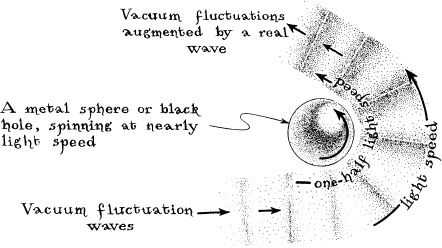
12.1 Zel’dovich’s mechanism by which vacuum fluctuations cause a spinning body to radiate.
The incoming wave is not a “real” wave, Zel’dovich explained, but rather a vacuum fluctuation. As this fluctuational wave sweeps around the spinning body, it behaves like a line of ice skaters making a turn: The outer skaters must whip around at high speed while the inner ones move much more slowly; similarly, the wave’s outer parts move at a very high speed, the speed of light, while its inner parts move much more slowly than light and, in fact, more slowly than the body’s surface is spinning. 8 In such a situation, Zel’dovich asserted, the rapidly spinning body will grab hold of the fluctuational wave and accelerate it, much like a small boy accelerating a slingshot as he swings it faster and faster. The acceleration feeds some of the body’s spin energy into the wave, amplifying it. The new, amplified portion of the wave is a “real wave” with positive total energy, while the original, unamplified portion remains a vacuum fluctuation with zero total energy (Box 12.4). The spinning body has thus used the vacuum fluctuation as a sort of catalyst for creating a real wave, and as a template for the shape of the real wave. This is similar, Zel’dovich pointed out, to the manner in which vacuum fluctuations cause a vibrating molecule to “spontaneously” emit light (Box 12.4).
Zel’dovich told me he had proved that a spinning metal sphere radiates in this way; his proof was based on the laws of quantum electrodynamics —that is, the well-known laws that arise from a marriage of quantum mechanics with Maxwell’s laws of electromagnetism. Though he did not have a similar proof that a spinning black hole will radiate, he was quite sure by analogy that it must. In fact, he asserted, a spinning hole will radiate not only gravitational waves, but also electromagnetic waves (photons 9 ), neutrinos, and all other forms of radiation that can exist in nature.
I was quite sure that Zel’dovich was wrong. Several hours later, with no agreement in sight, Zel’dovich offered me a wager. In the novels of Ernest Hemingway, Zel’dovich had read of White Horse scotch, an elegant and esoteric brand of whisky. If detailed calculations with the laws of physics showed that a spinning black hole radiates, then I was to bring Zel’dovich a bottle of White Horse scotch from America. If the calculations showed that there is no such radiation, Zel’dovich would give me a bottle of fine Georgian cognac.
I accepted the wager, but I knew it would not be settled quickly. To settle it would require understanding the marriage of general relativity and quantum mechanics far more deeply than anyone did in 1971.
Having made the wager, I soon forgot it. I have a lousy memory, and my own research was concentrated elsewhere. Zel’dovich, however, did not forget; several weeks after arguing with me, he wrote down his argument and submitted it for publication. The referee probably would have rejected his manuscript had it come from somebody else; his argument was too heuristic for acceptance. But Zel’dovich’s reputation carried the day; his paper was published—and hardly anyone paid any attention. Black-hole radiation just seemed horribly implausible.
A year later, at the Les. Houches summer school, we “experts” were still ignoring Zel’dovich’s idea. I don’t recall it being mentioned even onece. 10
I n September 1973, I was back in Moscow once again, this time accompanying Stephen Hawking and his wife Jane. This was Stephen’s first trip to Moscow since his student days. He, Jane, and Zel’dovich (our Soviet host), uneasy about how to cope in Moscow with Stephen’s special needs, thought it best that I, being familiar with Moscow and a close friend of Stephen’s and Jane’s, act as their companion, translator for physics conversations, and guide.
We stayed at the Hotel Rossiya, just off Red Square near the Kremlin Although we ventured out nearly every day to give lectures at one institute or another, or to visit a museum or the opera or ballet, our interactions with Soviet physicists occurred for the most part in the Hawkings’ two-room hotel suite, with its view of St. Basil’s Cathedral. One after another, the Soviet Union’s leading theoretical physicists came to the hotel to pay homage to Hawking and to converse.
Among the physicists who made repeated trips to Hawking’s hotel room were Zel’dovich and his graduate student Alexi Starobinsky. Hawking found Zel’dovich and Starobinsky as fascinating as they did him. On one visit, Starobinsky described Zel’dovich’s conjecture that a spinning black hole should radiate, described a partial marriage of quantum mechanics with general relativity that he and Zel’dovich had developed (based on earlier, pioneering work by Bryce DeWitt, Leonard Parker, and others), and then described a proof, using this partial marriage, that a spinning hole does, indeed, radiate. Zel’dovich was well on his way toward winning his bet with me.
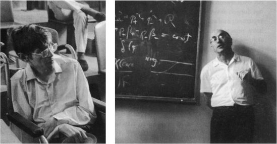
Left: Stephen Hawking listening to a lecture at the Les Houches summer school in summer 1972. Right: Yakov Borisovich Zel’dovich at the blackboard in his apartment in Moscow in summer 1971. [Photos by Kip Thorne.]
Of all the things Hawking learned from his conversations in Moscow, this one intrigued him most. However, he was skeptical of the manner in which Zel’dovich and Starobinsky had combined the laws of general relativity with the laws of quantum mechanics, so, after returning to Cambridge, he began to develop his own partial marriage of quantum mechanics and general relativity and use it to test Zel’-dovich’s claim that spinning holes should radiate.
In the meantime, several other physicists in America were doing the same thing, among them William Unruh (a recent student of Wheeler’s) and Don Page (a student of mine). By early 1974 Unruh and Page, each in his own way, had tentatively confirmed Zel’dovich’s prediction: A spinning hole should emit radiation until all of its spin energy has been used up and its emission stops. I would have to concede my bet.
Black Holes Shrink and Explode
T hen came a bombshell. Stephen Hawking, first at a conference in England and then in a brief technical article in the journal Nature, announced an outrageous prediction, a prediction that conflicted with Zel’dovich, Starobinsky, Page, and Unruh. Hawking’s calculations confirmed that a spinning black hole must radiate and slow its spin. However, they also predicted that, when the hole stops spinning, its radiation does not stop. With no spin left, and no spin energy left, the hole keeps on emitting radiation of all sorts (gravitational, electromagnetic, neutrino), and as it emits, it keeps on losing energy. Whereas the spin energy was stored in the swirl of space outside the horizon, the energy now being lost could come from only one place: from the hole’s interior!
Equally amazing, Hawking’s calculations predicted that the spectrum of the radiation (that is, the amount of energy radiated at each wavelength) is precisely like the spectrum of thermal radiation from a hot body. In other words, a black hole behaves precisely as though its horizon has a finite temperature, and that temperature, Hawking concluded, is proportional to the hole’s surface gravity. This (if Hawking was right) was incontrovertible proof that the Bardeen—Carter—Hawking laws of black-hole mechanics are the laws of thermodynamics in disguise, and that, as Bekenstein had claimed two years earlier, a black hole has an entropy proportional to its surface area.
Hawking’s calculations said more. Once the hole’s spin has slowed, its entropy and the area of its horizon are proportional to its mass squared, while its temperature and surface gravity are proportional to its mass divided by its area, which means inversely proportional to its mass. Therefore, as the hole continues to emit radiation, converting mass into outflowing energy, its mass goes down, its entropy and area go down, and its temperature and surface gravity go up. The hole shrinks and becomes hotter. In effect, the hole is evaporating.
A hole that has recently formed by stellar implosion (and that thus has a mass larger than about 2 Suns) has a very low temperature: less than 3 × 10 −8 degree above absolute zero (0.03 microkelvin). Therefore, the evaporation at first is very slow; so slow that the hole will require longer than 10 67 years (10 57 times the present age of the Universe) to shrink appreciably. However, as the hole shrinks and heats up, it will radiate more strongly and its evaporation will quicken. Finally, when the hole’s mass has been reduced to somewhere between a thousand tons and 100 million tons (we are not sure where), and its horizon has shrunk to a fraction the size of an atomic nucleus, the hole will be so extremely hot (between a trillion and 100,000 trillion degrees) that it will explode violently, in a fraction of a second.
T he world’s dozen experts on the partial marriage of general relativity with quantum theory were quite sure that Hawking had made a mistake. His conclusion violated everything then known about black holes. Perhaps his partial marriage, which differed from other people’s, was wrong; or perhaps he had the right marriage, but had made a mistake in his calculations.
For the next several years the experts minutely examined Hawking’s version of the partial marriage and their own versions, Hawking’s calculations of the waves from black holes and their own calculations. Gradually one expert after another came to agree with Hawking, and in the process they firmed up the partial marriage, producing a new set of physical laws. The new laws are called the laws of quantum fields in curved spacetime because they come from a partial marriage in which the black hole is regarded as a non—quantum mechanical, general relativistic, curved spacetime object, while the gravitational waves, electromagnetic waves, and other types of radiation are regarded as quantum fields —in other words, as waves that are subject to the laws of quantum mechanics and that therefore behave sometimes like waves and sometimes like particles (see Box 4.1). [A full marriage of general relativity and quantum theory, that is, the fully correct laws of quantum gravity, would treat everything, including the hole’s curved space-time, as quantum mechanical, that is, as subject to the uncertainty principle (Box 10.2), to wave/particle duality (Box 4.1), and to vacuum fluctuations (Box 12.4). We shall meet this full marriage and some of its implications in the next chapter.]
How was it possible to reach agreement on the fundamental laws of quantum fields in curved spacetime without any experiments to guide the choice of the laws? How could the experts claim near certainty that Hawking was right without experiments to check their claims? Their near certainty came from the requirement that the laws of quantum fields and the laws of curved spacetime be meshed in a totally consistent way. (If the meshing were not totally consistent, then the laws of physics, when manipulated in one manner, might make one prediction, for example, that black holes never radiate, and when manipulated in another manner, might make a different prediction, for example, that black holes must always radiate. The poor physicists, not knowing what to believe, might be put out of business.)
The new, meshed laws had to be consistent with general relativity’s laws of curved spacetime in the absence of quantum fields and with the laws of quantum fields in the absence of spacetime curvature. This and the demand for a perfect mesh, analogous to the demand that the rows and columns of a crossword puzzle mesh perfectly, turned out to determine the form of the new laws almost 11 completely. If the laws could be meshed consistently at all (and they must be, if the physicists’ approach to understanding the Universe makes any sense), then they could be meshed only in the manner described by the new, agreed-upon laws of quantum fields in curved spacetime.
The requirement that the laws of physics mesh consistently is often used as a tool in the search for new laws. However, this consistency requirement has rarely exhibited such great power as here, in the arena of quantum fields in curved spacetime. For example, when Einstein was developing his laws of general relativity (Chapter 2 ), considerations of consistency could not and did not tell him his starting premise, that gravity is due to a curvature of spacetime; this starting premise came largely from Einstein’s intuition. However, with this premise in hand, the requirement that the new general relativistic laws mesh consistently with Newton’s laws of gravity when gravity is weak, and with the laws of special relativity when there is no gravity at all, determined the forms of the new laws almost uniquely; for example, it was the key to Einstein’s discovery of his field equation.
I n September 1975,I returned to Moscow for my fifth visit, bearing a bottle of White Horse scotch for Zel’dovich. To my surprise, I discovered that, although all the Western experts by now had agreed that Hawking was right and black holes can evaporate, nobody in Moscow believed Hawking’s calculations or conclusions. Although several confirmations of Hawking’s claims, derived by new, completely different methods, had been published during 1974 and 1975, those confirmations had had little impact in the U.S.S.R. Why? Because Zel’dovich and Starobinsky, the greatest Soviet experts, were disbelievers: They continued to maintain that, after a radiating black hole has lost all its spin, it must stop radiating, and it therefore cannot evaporate completely. I argued with Zel’dovich and Starobinsky, to no avail; they knew so much more about quantum fields in curved spacetime than I that although (as usual) I was quite sure I had truth on my side, I could not counter their arguments.
My return flight to America was scheduled for Tuesday, 23 September. On Monday evening, as I was packing my bags in my tiny room at the University Hotel, the telephone rang. It was Zel’dovich: “Come to my flat, Kip! I want to talk about black-hole evaporation!” Tight for time, I sought a taxi in front of the hotel. None was in sight, so in standard Muscovite fashion I flagged down a passing motorist and offered him five rubles to take me to Number 2B Vorobyevskoye Shosse. He nodded agreement and we were off, down back streets I had never traveled. My fear of being lost abated when we swung onto Vorobyevskoye Shosse. With a grateful “Spasibo!” I alighted in front of 2B, jogged through the gate and forested grounds, into the building, and up the stairs to the second floor, southwest corner.
Zel’dovich and Starobinsky greeted me at the door, grins on their faces and their hands above their heads. “We give up; Hawking is right; we were wrong!” For the next hour they described to me how their version of the laws of quantum fields in a black hole’s curved spacetime, while seemingly different from Hawking’s, was really completely equivalent. They had concluded black holes cannot evaporate because of an error in their calculations, not because of wrong laws. With the error corrected, they now agreed. There is no escape. The laws require that black holes evaporate.
T here are several different ways to picture black-hole evaporation, corresponding to the several different ways to formulate the laws of quantum fields in a black hole’s curved spacetime. However, all the ways acknowledge vacuum fluctuations as the ultimate source of the outflowing radiation. Perhaps the simplest pictorial description is one based on particles rather than waves:
Vacuum fluctuations, like “real,” positive-energy waves, are subject to the laws of wave/particle duality (Box 4.1); that is, they have both wave aspects and particle aspects. The wave aspects we have met already (Box 12.4): The waves fluctuate randomly and unpredictably, with positive energy momentarily here, negative energy momentarily there, and zero energy on average. The particle aspect is embodied in the concept of virtual particles, that is, particles that flash into existence in pairs (two particles at a time), living momentarily on fluctuational energy borrowed from neighboring regions of space, and that then annihilate and disappear, giving their energy back to the neighboring regions. For electromagnetic vacuum fluctuations, the virtual particles are virtual photons; for gravitational vacuum fluctuations, they are virtual gravitons. 12
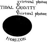
12.2 The mechanism of black-hole evaporation, as viewed by someone who is falling into the hole. Left: A black hole’s tidal gravity pulls a pair of virtual photons apart, thereby feeding energy into them. Right: The virtual photons have acquired enough energy from tidal gravity to materialize, permanently, into real photons, one of which escapes from the hole while the other falls toward the hole’s center.
The manner in which vacuum fluctuations cause black holes to evaporate is depicted in Figure 12.2. On the left is shown a pair of virtual photons near a black hole’s horizon, as viewed in the reference frame of someone who is falling into the hole. The virtual photons can separate from each other easily, so long as they both remain in a region where the electromagnetic field has momentarily acquired positive energy. That region can have any size from tiny to huge, since vacuum fluctuations occur on all length scales; however, the region’s size will always be about the same as the wavelength of its fluctuating electromagnetic wave, so the virtual photons can move apart by only about one wavelength. If the wavelength happens to be about the same as the hole’s circumference, then the virtual photons can easily separate from each other by a quarter of the circumference, as shown in the figure.
Tidal gravity near the horizon is very strong; it pulls the virtual photons apart with a huge force, thereby feeding great energy into them, as seen by the infalling observer who is halfway between the photons. The increase in photon energy is sufficient, by the time the photons are a quarter of a horizon circumference apart, to convert them into real long-lived photons (right half of Figure 12.2), and have enough energy left over to give back to the neighboring, ‘negative-energy regions of space. The photons, now real, are liberated from each other. One is inside the horizon and lost forever from the external Universe. The other escapes from the hole, carrying away the energy (that is, the mass 13 ) that the hole’s tidal gravity gave to it. The hole, with its mass reduced, shrinks a bit.
This mechanism of emitting particles does not depend at all on the fact that the particles were photons, and their associated waves were electromagnetic. The mechanism will work equally well for all other forms of particle/wave (that is, for all other types of radiation—gravitational, neutrino, and so forth), and therefore a black hole radiates all types of radiation.
Before the virtual particles have materialized into real particles, they must stay closer together than roughly the wavelength of their waves. To acquire enough energy from the hole’s tidal gravity to materialize, however, they must get as far apart as about a quarter of the circumference of the hole. This means that the wavelengths of the particle/waves that the hole emits will be about one-fourth the hole’s circumference in size, and larger.
A black hole with mass twice as large as the Sun has a circumference of about 35 kilometers, and thus the particle/waves that it emits have wavelengths of about 9 kilometers and larger. These are enormous wavelengths compared to light or ordinary radio waves, but not much different from the lengths of the gravitational waves that the hole would emit if it were to collide with another hole.
D uring the early years of his career, Hawking tried to be very careful and rigorous in his research. He never asserted things to be true unless he could give a nearly airtight proof of them. However, by 1974 he had changed his attitude: “I would rather be right than rigorous,” he told me firmly. Achieving high rigor requires much time. By 1974 Hawking had set for himself goals of understanding the full marriage of general relativity with quantum mechanics, and understanding the origin of the Universe—goals that to achieve would require enormous amounts of time and concentration. Perhaps feeling more finite than other people feel because of his life-shortening disease, Hawking felt he could not afford to dally with his discoveries long enough to achieve high rigor, nor could he afford to explore all the important features of his discoveries. He must push on at high speed.
Thus it was that Hawking, in 1974, having proved firmly that a black hole radiates as though it had a temperature proportional to its surface gravity, went on to assert, without real proof, that all of the other similarities between the laws of black-hole mechanics and the laws of thermodynamics were more than a coincidence: The black-hole laws are the same thing as the thermodynamic laws, but in disguise. From this assertion and his firmly proved relationship between temperature and surface gravity, Hawking inferred a precise relationship between the hole’s entropy and its surface area: The entropy is 0.10857 ... times 14 the surface area, divided by the Planck–Wheeler area. In other words, a 10-solar-mass, nonspinning hole has an entropy of 4.6 × 10 78 , which is approximately the same as Bekenstein’s conjecture.
Bekenstein, of course, was sure Hawking was right, and he glowed with pleasure. By the end of 1975, Zel’dovich, Starobinsky, I, and Hawking’s other colleagues were also strongly inclined to agree. However, we would not feel fully satisfied until we understood the precise nature of a black hole’s enormous randomness. There must be 10 4.6 × 10 78 ways to distribute something inside the black hole, without changing its external appearance (its mass, angular momentum, and charge), but what was that something? And how, in simple physical terms, could one understand the thermal behavior of a black hole—the fact that the hole behaves just like an ordinary body with temperature? As Hawking moved on to research on quantum gravity and the origin of the Universe, Paul Davies, Bill Unruh, Robert Wald, James York, I, and many others of his colleagues zeroed in on these issues. Gradually over the next ten years we arrived at the new understanding embodied in Figure 12.3.
Figure 12.3a depicts a black hole’s vacuum fluctuations, as viewed by observers falling inward through the horizon. The vacuum fluctuations consist of pairs of virtual particles. Occasionally tidal gravity manages to give one of the plethora of pairs sufficient energy for its two virtual particles to become real, and for one of them to escape from the hole. This was the viewpoint on vacuum fluctuations and black-hole evaporation discussed in Figure 12.2.
Figure 12.3b depicts a different viewpoint on the hole’s vacuum fluctuations, the viewpoint of observers who reside just above the hole’s horizon and are forever at rest relative to the horizon. To prevent themselves from being swallowed by the hole, such observers must accelerate hard, relative to falling observers—using a rocket engine or hanging by a rope. For this reason, these observers’ viewpoint is called the “accelerated viewpoint.” It is also the viewpoint of the “membrane paradigm” (Chapter 11 ).
Surprisingly, from the accelerated viewpoint, the vacuum fluctuations consist not of virtual particles flashing in and out of existence, but rather of real particles with positive energies and long lives; see Box 12.5. The real particles form a hot atmosphere around the hole, much like the atmosphere of the Sun. Associated with these real particles are real waves. As a particle moves upward through the atmosphere, gravity pulls on it, reducing its energy of motion; correspondingly, as a wave moves upward, it becomes gravitationally redshifted to longer and longer wavelengths (Figure 12.3b).
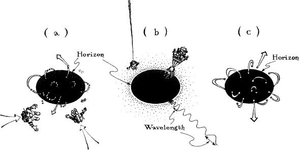
12.3 (a) Observers falling into a black hole (the two little men in space suits) see vacuum fluctuations near the hole’s horizon to consist of pairs of virtual particles, (b) As viewed by observers just above the horizon and at rest relative to the horizon (the little man hanging by a rope and the little man blasting his rocket engine), the vacuum fluctuations consist of a hot atmosphere of real particles; this is the “accelerated viewpoint.” (c) The atmosphere’s particles, in the accelerated viewpoint, appear to be emitted by a hot, membrane-like horizon. They fly upward short distances, and most are then pulled back into the horizon. However, a few of the particles manage to escape the hole’s grip and evaporate into outer space.
Box 12.5
Acceleration Radiation
In 1975, Wheeler’s recent student William Unruh, and independently Paul Davies at King’s College, London, discovered (using the laws of quantum fields in curved spacetime) that accelerated observers just above a black hole’s horizon must see the vacuum fluctuations there not as virtual pairs of particles but rather as an atmosphere of real particles, an atmosphere that Unruh called “acceleration radiation.”
This startling discovery revealed that the concept of a real particle is relative, not absolute; that is, it depends on one’s reference frame. Observers in freely falling frames who plunge through the hole’s horizon see no real particles outside the horizon, only virtual ones. Observers in accelerated frames who, by their acceleration, remain always above the horizon see a plethora of real particles.
How is this possible? How can one observer claim that the horizon is surrounded by an atmosphere of real particles and the other that it is not? The answer lies in the fact that the virtual particles’ vacuum fluctuational waves are not confined solely to the region above the horizon; part of each fluctuational wave is inside the horizon and part is outside.
• The freely falling observers, who plunge through the horizon, can see both parts of the vacuum fluctuational wave, the part inside the horizon and the part outside; so such observers are well aware (by their measurements) that the wave is a mere vacuum fluctuation and correspondingly that its particles are virtual, not real.
• The accelerated observers, who remain always outside the horizon, can see only the outside part of the vacuum fluctuational wave, not the inside part; and correspondingly, by their measurements they are unable to discern that the wave is a mere vacuum fluctuation accompanied by virtual particles. Seeing only a part of the fluctuational wave, they mistake it for “the real thing”—a real wave accompanied by real particles, and as a result their measurements reveal all around the horizon an atmosphere of real particles.
That this atmosphere’s real particles can gradually evaporate and fly off into the external Universe (Figure 12.3c) is an indication that the viewpoint of the accelerated observers is just as correct, that is, just as valid, as that of the freely falling observers: What the freely falling observers see as virtual pairs converted into real particles by tidal gravity, followed by evaporation of one of the real particles, the accelerated observers see simply as the evaporation of one of the particles that was always real and always populated the black hole’s atmosphere. Both viewpoints are correct; they are the same physical situation, seen from two different reference frames.
Figure 12.3c shows the motion of a few of the particles in a black-hole atmosphere, from the accelerated viewpoint. The particles appear to be emitted by the horizon; most fly upward a short distance and are then pulled back down to the horizon by the hole’s strong gravity, but a few manage to escape the hole’s grip. The escaping particles are the same ones as the infalling observers see materialize from virtual pairs (Figure 12.3a). They are Hawking’s evaporating particles.
From the accelerated viewpoint, the horizon behaves like a high-temperature, membrane-like surface; it is the membrane of the “membrane paradigm” described in Chapter 11 . Just as the Sun’s hot surface emits particles (for example, the photons that make daylight on Earth), so the horizon’s hot membrane emits particles: the particles that make up the hole’s atmosphere, and the few that evaporate. The gravitational redshift reduces the particles’ energy as they fly upward from the membrane, so although the membrane itself is extremely hot, the evaporating radiation is much cooler.
The accelerated viewpoint not only explains the sense in which a black hole is hot, it also accounts for the hole’s enormous randomness. The following thought experiment (invented by me and my postdoc, Wojciech Zurek) explains how.
Throw into a black hole’s atmosphere a small amount of material containing some small amount of energy (or, equivalently, mass), angular momentum (spin), and electric charge. From the atmosphere this material will continue on down through the horizon and into the hole. Once the material has entered the hole, it is impossible by examining the hole from outside to learn the nature of the injected material (whether it consisted of matter or of antimatter, of photons and heavy atoms, or of electrons and positrons), and it is impossible to learn just where the material was injected. Because a black hole has no “hair,” all one can discover, by examining the hole from outside, are the total amounts of mass, angular momentum, and charge that entered the atmosphere.
Ask how many ways those amounts of mass, angular momentum, and charge could have been injected into the hole’s hot atmosphere. This question is analogous to asking how many ways the child’s toys could have been distributed over the tiles in the playroom of Box 12.3, and correspondingly, the logarithm of the number of ways to inject must be the increase in the atmosphere’s entropy, as described by the standard laws of thermodynamics. By a fairly simple calculation, Zurek and I were able to show that this increase in thermodynamic entropy is precisely equal to ¼ times the increase in the horizon’s area, divided by the Planck–Wheeler area; that is, it is precisely the increase in the horizon’s area in disguise, the same disguise that Hawking inferred, in 1974, from the mathematical similarity of the laws of black-hole mechanics and the laws of thermodynamics.
The outcome of this thought experiment can be expressed succinctly as follows: A black hole’s entropy is the logarithm of the number of ways that the hole could have been made. This means that there are 10 4.6 × 10 78 different ways to make a 10-solar-mass black hole whose entropy is 4.6 × 10 78 . This explanation of the entropy was originally conjectured by Bekenstein in 1972, and a highly abstract proof was given by Hawking and his former student, Gary Gibbons, in 1977.
The thought experiment also shows the second law of thermodynamics in action. The energy, angular momentum, and charge that one throws into the hole’s atmosphere can have any form at all; for example, they might be the roomful of air wrapped up in a bag, which we met earlier in this chapter while puzzling over the second law. When the bag is thrown into the hole’s atmosphere, the entropy of the external Universe is reduced by the amount of entropy (randomness) in the bag. However, the entropy of the hole’s atmosphere, and thence of the hole, goes up by more than the bag’s entropy, so the total entropy of hole plus external Universe goes up. The second law of thermodynamics is obeyed.
Similarly, it turns out, when the black hole evaporates some particles, its own surface area and entropy typically go down; but the particles get distributed randomly in the external Universe, increasing its entropy by more than the hole’s entropy loss. Again the second law is obeyed.
H ow long does it take for a black hole to evaporate and disappear? The answer depends on the hole’s mass. The larger the hole, the lower its temperature, and thus the more weakly it emits particles and the more slowly it evaporates. The total lifetime, as worked out by Don Page in 1975 when he was jointly my student and Hawking’s, is 1.2 × 10 67 years if the hole’s mass is twice that of the Sun. The lifetime is proportional to the cube of the hole’s mass, so a 20-solar-mass hole has a life of 1.2 × 10 70 years. These lifetimes are so enormous compared to the present age of the Universe, about 1 × 10 10 years, that the evaporation is totally irrelevant for astrophysics. Nevertheless, the evaporation has been very important for our understanding of the marriage between general relativity and quantum mechanics; the struggle to understand the evaporation taught us the laws of quantum fields in curved spacetime.
Holes far less massive than 2 Suns, if they could exist, would evaporate far more rapidly than 10 67 years. Such small holes cannot be formed in the Universe today because degeneracy pressures and nuclear pressures prevent small masses from imploding, even if one squeezes them with all the force the present-day Universe can muster (Chapters 4 and 5 ). However, such holes might have formed in the big bang, where matter experienced densities and pressures and gravitational squeezes that were enormously higher than in any modern-day star.
Detailed calculations by Hawking, Zel’dovich, Novikov, and others have shown that tiny lumps in the matter emerging from the big bang could have produced tiny black holes, if the lumps’ matter had a rather soft equation of state (that is, had only small increases of pressure when squeezed). Powerful squeezing by other, adjacent matter in the very early Universe, like the squeezing of carbon in the jaws of a powerful anvil to form diamond, could have made the tiny lumps implode to produce tiny holes.
A promising way to search for such tiny primordial black holes is by searching for the particles they produce when they evaporate. Black holes weighing less than about 500 billion kilograms (5 × 10 14 grams, the weight of a modest mountain) should have evaporated completely away by now, and black holes a few times heavier than this should still be evaporating strongly. Such black holes have horizons about the size of an atomic nucleus.
A large portion of the energy emitted in the evaporation of such holes should now be in the form of gamma rays (high-energy photons) traveling randomly through the Universe. Such gamma rays do exist, but in amounts and with properties that are readily explained in other ways. The absence of excess gamma rays tells us (according to calculations by Hawking and Page) that there now are no more than about 300 tiny, strongly evaporating black holes in each cubic light-year of space; and this, in turn, tells us that matter in the big bang cannot have had an extremely soft equation of state.
Skeptics will argue that the absence of excess gamma rays might have another interpretation: Perhaps many small black holes were formed in the big bang, but we physicists understand quantum fields in curved spacetime far less well than we think we do, and thus we are misleading ourselves when we believe that black holes evaporate. I and my colleagues resist such skepticism because of the seeming perfection with which the standard laws of curved spacetime and the standard laws of quantum fields mesh to give us a nearly unique set of laws for quantum fields in curved spacetime. Nevertheless, we would feel rather more comfortable if astronomers could find observational evidence of black-hole evaporation.
1. It might seem counterintuitive that Hawking’s area-increase theorem permits any of the holes’ mass at all to be emitted as gravitational waves. Readers comfortable with algebra may find satisfaction in the example of two nonspinning holes that coalesce to produce a single, larger nonspinning hole. The surface area of a nonspinning hole is proportional to the square of its horizon circumference, which in turn is proportional to the square of the hole’s mass. Thus, Hawking’s theorem insists that the sum of the squares of the initial holes’ masses must be less than the square of the final hole’s mass. A little algebra shows that this constraint on the masses permits the final hole’s mass to be less than the sum of the initial holes’ masses, and thus permits some of the initial masses to be emitted as gravitational waves.
2. A more precise definition of the apparent horizon is given in Box 12.1 below.
3. The laws of quantum mechanics guarantee that the number of ways to distribute the atoms and molecules is always finite, and never infinite. In defining the entropy, physicists often multiply the logarithm of this number of ways by a constant that will be irrelevant to us, loge10 × k , where loge10 is the “natural logarithm” of 10, that is, 2.30258 . . . , and k is “Boltzmann’s constant,” 1.38062 × 10 −16 erg per degree Celsius. Throughout this book I shall ignore this constant.
4. This Planck-Wheeler area is given by the formula Għ /c 3 , where G = 6.670 × 10 −8 dyne-cehtimeter 2 /gram 2 is Newton’s gravitation constant, ħ = 1.055 × 1 0- 27 erg-second is Planck’s quantum mechanical constant, and c = 2.998 × 10 10 centimeter/second is the speed of light. For related issues, see Footnote 2 in Chapter 13 , Footnote 6 in Chapter 14 , and the associated discussions in the text of those chapters.
5. The logarithm of 10 1079 is 10 79 (Bekenstein’s conjectured entropy). Note that 10 10 79 is a 1 with 10 79 zeroes after it, that is, with nearly as many zeroes as there are atoms in the Universe.
6. Vorobyevskoye Shosse has since been renamed Kosygin Street, and its buildings have been renumbered. In the late 1980s Mikhail Gorbachev had a home at Number 10, several doors west of Zel’dovich.
7. See the last section of Chapter 1 : “The Nature of Physical Law.”
8. In technical language, the outer parts are in the “radiation zone” while the inner parts are in the “near zone.”
9. Recall that photons and electromagnetic waves are different aspects of the same thing; see the discussion of wave/particle duality in Box 4.1.
10. This lack of interest was all the more remarkable because in the meantime, Charles Misner in America had shown that real waves (as opposed to Zel’dovich’s vacuum fluctuations) can be amplified by a spinning hole in a manner analogous to Figure 12.1, and this amplification—to which Misner gave the name “superradiance”-—-was generating great interest.
11. The “almost” takes care of certain ambiguities in a procedure called “renormalization,” by which one computes the net energy carried by vacuum fluctuations. These ambiguities, which were identified and codified by Robert Wald (a former student of Wheeler’s), do not influence a black hole’s evaporation, and they probably will not be resolved until the full quantum theory of gravity is in hand.
12. Some readers may already be familiar with these concepts in the context of matter and antimatter, for example, an electron (which is a particle of matter) and a positron (its antiparticle). Just as the electromagnetic field is the field aspect of a photon, so also there exists an electron field which is the field aspect of the electron and the positron. At locations where the electron field’s vacuum fluctuations are momentarily large, a virtual electron and a virtual positron are likely to flash into existence, as a pair; when the field fluctuates down, the electron and positron are likely to annihilate each other and disappear. The photon is its own antiparticle, so virtual photons flash in and out of existence in pairs, and similarly for gravitons
13. Recall that, since mass and energy are totally convertible into each other, they are really just different names for the same concept.
14. The peculiar factor 0.10857 ... is actually 1/(4logel0), where loge10 = 2.30258 . . . results from my choice of “normalization” of the entropy; see Footnote 3 on page 423 .